Good afternoon, dear readers! Quite a lot of materials have been written about this method of segmentation of customers by age of purchases, frequency and amount of transactions. On the Internet, you can easily find publications describing the theory and practice of rfm analysis. It can be executed both on the platform of a spreadsheet editor (with a small amount of data), and using sql queries or using Python / R thematic libraries. The methodology of all examples is the same, the discrepancy will be only in the details. For example, the order of assigning numbers to segments or the principle of division into groups. In view of all of the above, it will be difficult for me to bring novelty to this topic. In this article, I will only try to draw your attention to some points that can help novice data analysts.
To demonstrate how the scripts work, I chose PostgreSQL and JupyterLab from Anaconda. All code examples that you will see in the post can be found on GitHub ( link ). Data for analysis was taken from the Kaggle portal ( link ).
Before loading the dataset into the database, examine the data if you are not sure of its quality in advance. Particular attention should be paid to columns with dates, gaps in records, incorrect definition of the type of fields. For the sake of simplicity in the demo, I have also rejected the item return entries.
import pandas as pd
import numpy as np
import datetime as dt
pd.set_option('display.max_columns', 10)
pd.set_option('display.expand_frame_repr', False)
df = pd.read_csv('dataset.csv', sep=',', index_col=[0])
#
df.columns = [_.lower() for _ in df.columns.values]
# -
df['invoicedate'] = pd.to_datetime(df['invoicedate'], format='%m/%d/%Y %H:%M')
df['invoicedate'] = df['invoicedate'].dt.normalize()
#
df_for_report = df.loc[(~df['description'].isnull()) &
(~df['customerid'].isnull()) &
(~df['invoiceno'].str.contains('C', case=False))]
#
convert_dict = {'invoiceno': int, 'customerid': int, 'quantity': int, 'unitprice': float}
df_for_report = df_for_report.astype(convert_dict)
#
# print(df_for_report.head(3))
# print(df_for_report.dtypes)
# print(df_for_report.isnull().sum())
# print(df_for_report.info())
# csv
df_for_report.to_csv('dataset_for_report.csv', sep=";", index=False)
The next step is to create a new table in the database. This can be done both in the graphical editor mode using the pgAdmin utility, and using Python code.
import psycopg2
#
conn = psycopg2.connect("dbname='db' user='postgres' password='gfhjkm' host='localhost' port='5432'")
print("Database opened successfully")
#
cursor = conn.cursor()
with conn:
cursor.execute("""
DROP TABLE IF EXISTS dataset;
""")
cursor.execute("""
CREATE TABLE IF NOT EXISTS dataset (
invoiceno INTEGER NOT NULL,
stockcode TEXT NOT NULL,
description TEXT NOT NULL,
quantity INTEGER NOT NULL,
invoicedate DATE NOT NULL,
unitprice REAL NOT NULL,
customerid INTEGER NOT NULL,
country TEXT NOT NULL);
""")
print("Operation done successfully")
#
cursor.close()
conn.close()
, . PostgreSQL. , . Pandas.
import psycopg2
from datetime import datetime
start_time = datetime.now()
#
conn = psycopg2.connect("dbname='db' user='postgres' password='gfhjkm' host='localhost' port='5432'")
print("Database opened successfully")
#
cursor = conn.cursor()
# .
with open('dataset_for_report.csv', 'r') as f:
next(f)
cursor.copy_from(f, 'dataset',sep=';', columns=('invoiceno', 'stockcode', 'description', 'quantity',
'invoicedate','unitprice', 'customerid', 'country'))
conn.commit()
f.close()
print("Operation done successfully")
#
cursor.close()
conn.close()
end_time = datetime.now()
print('Duration: {}'.format(end_time - start_time))
rfm-. , , sql. , ( Hadoop ). rfm- : , .
. , ( Pandas – cut qcut) . , . , , - . -, . , . , : , . , -.
-- rfm-
create function func_recency(days integer) returns integer as $$
select case when days<90 then 1
when (days>=90) and (days<=180) then 2
else 3
end;
$$ language sql;
create function func_frequency(transactions integer) returns integer as $$
select case when transactions>50 then 1
when (transactions>=10) and (transactions<=50) then 2
else 3
end;
$$ language sql;
create function func_monetary(amount integer) returns integer as $$
select case when amount>10000 then 1
when (amount>=1000) and (amount<=10000) then 2
else 3
end;
$$ language sql;
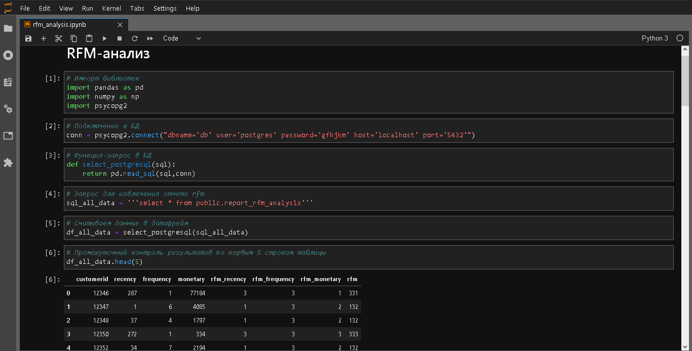
, rfm-. . . , , . , , , , , – . , rfm-. sql- BI JupyterLab.
-- rfm-
select d3.*, concat(d3.rfm_recency,d3.rfm_frequency,d3.rfm_monetary) as rfm
from
(select d2.customerid,
date('2011-11-01')- max(d2.invoicedate) as recency,
cast(count(distinct(d2.invoiceno)) as integer) as frequency,
cast(sum(d2.amount) as integer) as monetary,
func_recency(date('2011-11-01')- max(d2.invoicedate)) as rfm_recency,
func_frequency(cast(count(distinct(d2.invoiceno))as integer)) as rfm_frequency,
func_monetary(cast(sum(d2.amount)as integer)) as rfm_monetary
from
(select d.*, d.quantity * d.unitprice as amount
from public.dataset as d
where d.invoicedate < date('2011-11-01')) as d2
group by d2.customerid
order by d2.customerid) as d3;
, . -, rfm- , , -, , , .
? . . , - . , , 50 , . ? , . , , . , , , 5000 , . 500 , . Sql- . , JupyterLab .
-- , ,
select r.rfm,
sum(r.monetary) as total_amount,
count(r.rfm) as count_customer,
cast(avg(r.monetary/r.frequency) as integer) as avg_check
from public.report_rfm_analysis as r
group by r.rfm;
. , . -, . - , 70% . .
--
select d2.rfm,
d2.country,
cast(sum(d2.amount) as integer) as amount_country,
round(cast(sum(d2.amount)/sum(sum(d2.amount))over(partition by d2.rfm)*100 as numeric),2) as percent_total_amount
from
(select d.*, d.quantity * d.unitprice as amount, r.rfm
from public.dataset as d left join
public.report_rfm_analysis as r on d.customerid = r.customerid
where d.invoicedate < date('2011-11-01')) as d2
group by d2.rfm, d2.country
order by d2.rfm, sum(d2.amount)desc;
. : , -7 , -3 , . . , , . , - , - , , . . If the communication with the client is necessarily the most targeted. To demonstrate this approach, I implemented the calculation of the top 3 days in terms of sales in the context of segment-country.
--
create function func_day_of_week(number_day integer) returns text as $$
select (string_to_array('sunday,monday,tuesday,wednesday,thursday,friday,saturday',','))[number_day];
$$ language sql;
-- -3 -
select d4.rfm, d4.country, max(d4.top) as top_3_days
from
(select d3.rfm, d3.country, string_agg(d3.day_of_week,', ')over(partition by d3.rfm, d3.country) as top
from
(select d2.rfm, d2.country, d2.day_of_week,sum(d2.amount) as total_amount,
row_number ()over(partition by d2.rfm, d2.country order by d2.rfm, d2.country, sum(d2.amount)desc)
from
(select r.rfm,
d.country,
func_day_of_week(cast(to_char(d.invoicedate, 'D') as integer)) as day_of_week,
d.quantity * d.unitprice as amount
from public.dataset as d left join public.report_rfm_analysis as r on d.customerid = r.customerid
where d.invoicedate < date('2011-11-01')) as d2
group by d2.rfm, d2.country, d2.day_of_week
order by d2.rfm, d2.country, sum(d2.amount) desc) as d3
where d3.row_number <= 3) as d4
group by d4.rfm, d4.country
Brief conclusions . RFM analysis and auxiliary calculations for it are most conveniently performed by combining sql and Python notebooks. When segmenting customers, it is important to take into account the business area, marketing policy and advertising goals. An RFM report does not give the whole picture, so it is best to accompany it with auxiliary calculations.
That's all. All health, good luck and professional success!