Next, we will try to construct a discount curve for the Swedish krona.
This post is an adapted version of my third video lecture " Building the Discount Curve " as part of the Finmath for Fintech course.
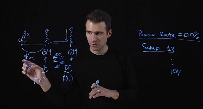
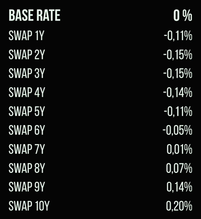
So, our discount curve for the krona will be the overnight rates for each day. The first thing we know is the so-called base rate - the rate on short deposits (loans). Further, there are known swaps ranging from one year to thirty years. To illustrate the method, we will plot a curve up to ten years. The current market data values can be seen in this image:
To start plotting the curve, we need to make a few assumptions.
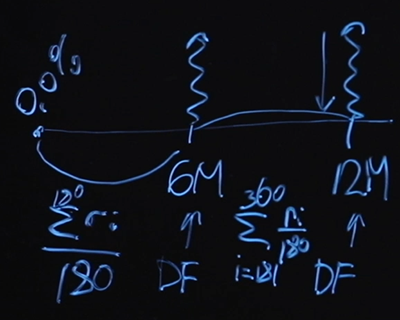
Let's assume for the sake of simplicity that our swaps are fix floating swaps with a periodicity of payments every six months. Below is the diagram for a one year swap. We know that at the beginning the base rate is zero percent. To calculate a fair swap price, we need to know the value of the six month discount factor and the 12 month discount factor. What will we have as a floating "leg"? Suppose that as it we will pay the average overnight value for each of the ranges. That is, the value of the floating "leg" up to six months - this will be the average overnight value over 180 days. The floating leg for the 12 month point will be the same, only here there will be a summation from day 181 to day 360.
This averaging method is widely known. It's called the overnight index swap and is used very often in market products. The floating leg is here defined as the average over the period.
We know the base rate and the cost of the swap. Obviously, if we write the formula for a fair price "head on", then we will have too many unknowns. We do not know the discount factor for 6 months, the discount factor for 12 months, and we do not know the values of interest rates except for one - the very first. Too many unknowns and just one equation.

The following hypothesis will help us in solving this problem. We know the interest rate at point zero - this is the base rate. We will assume that our interest rates are changing linearly. Let's designate as X the value of the interest rate at the point of 12 months.
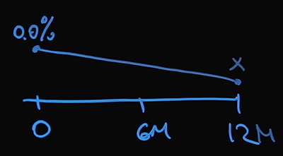
At 6 months it will be X / 2 (the arithmetic mean between zero and X), and we can find the value of the interest rate on any arbitrary day. And there is nothing difficult in calculating our floating interest rate at points 6 and 12 months:
Now let's move on to the discount factors. We use a discount curve based on the overnight rate. Therefore, the discount factor at the point six months is the product of 180 discount factors at each point, and this will obviously be some kind of function of X. The
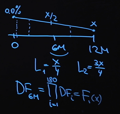
discount factor at the point 12 months is constructed in a similar way with the only difference that I need more multipliers. This will also be some function of X.

So, the discount factors are expressed in terms of X, there are also the first and second values of the floating rate. Let's move on to writing the equation. We know the value of the swap price, let's say it is equal to P. Recall the equation for the fair price. We need to multiply P by the discount factor at the point of twelve months and equate to the following sum:

Let me remind you that the discount factor for one day will be determined by the following formula:
where r i is the value of the interest rate. I use the number 360 on the assumption that there are 360 days in a year (this is a very common convention for calendars). At any given point, we know how to express the discount factor, r i expressed in terms of X, using linear interpolation. Our equation turns out to be with only one unknown, and it can be solved using numerical methods. How to do this - see the Python code .
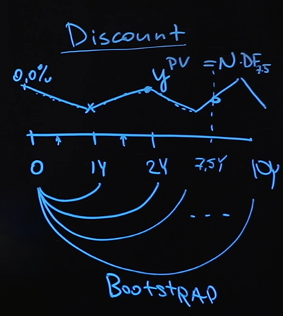
So, we know how to find the value of our rate at the point 1 year. Using the assumption of linear interpolation and based on the swap value that we know from the market, we will find our value for X. Here we plotted the first section of our curve:

Now, to calculate the swap price for two years, we need the value at the point 6 months, 12 months, 18 months and 2 years. We will use exactly the same assumption as last time. Let's call the value of the desired rate Y and also use the assumption about the interpolation line, restoring the second section of the curve. Thus, step by step, we will reach the end - to the point of 10 years.

This method is called bootstrap . It is not perfect or the only correct one, but it is simple enough to implement and understand - the bootstrap method is great as a starting level.

We found the discount curve. What does it give us? Formally speaking, these are the values of the overnight rate at any point in the future up to ten years. You probably ask: "Who needs it?" Indeed, it is difficult to imagine a scenario when a client comes to you and says: "I want to open a one-day deposit, which will start in 567 days." This is a rather incomprehensible situation, and one should not perceive the constructed curve in such a direct form.
Let's imagine that we have some kind of payment in the future, say seven and a half years. Question: how do we know its current value?
This is exactly the question that the discount curve will answer. We will go along each point of the curve, calculate the discount factor at each point and end our journey at the point for seven and a half years, find the resulting discount factor, multiply by the payment - this will be an honest price.
The model that I used, namely what floating rates I took, how I interpolated intermediate values, and in general the fact that I chose interpolation was very much determined by what kind of data I have. I had very little data - just one base rate and swap values. If more data is available to me, or it is different, then most likely I will change the model. But the bootstrap method (when you plot the curve first on a short section, and then plot further and further, relying on the previously obtained values) still applies.
Now let's remember that in addition to the discount curves, we need LIBOR curves (TIBOR, EURIBOR, etc.). The difference will be in what tools we add to our model for calculation. We will look for contracts containing LIBOR and in a similar way, using the bootstrap method, we will reconstruct the LIBOR curve.
If you have to build a real LIBOR curve, be very careful about what tools you use to build it, carefully evaluate the model that you will use. In this case, I used overnight discounting, but a different method is needed to construct the LIBOR curve. Most likely, the discounting will be every three months or six, depending on the instrument. If you have enough data, you can plot a LIBOR curve, EURIBOR curve, TIBOR curve, and any other.
If a client comes to you with the words: “I want an interest rate swap not for ten years, but for 134 months, during which I will pay floating LIBOR every 25 days,” this is not a problem. We have a LIBOR curve, we use the interpolation assumption, we can restore the LIBOR value at any point. We know the value of the discount curve at each point, we can also calculate all payments and find the very price of the fixed "leg" that balances these floating payments. Thus, you can find the fair price values for absolutely any instrument by plotting several curves.
So let's go over the highlights again. I took the available data and formulated a few assumptions. First, the payment schedule: how often, how often, each party pays a fixed leg and a floating leg. Second, how will I calculate the bet on the floating leg? The third assumption is about linear bet interpolation. Using all three of these assumptions, I formulated several nonlinear equations, which I solved numerically. Jupyter notebook can be found here. Sequentially, starting from the shortest segment of one year, then two years, three, etc., I reconstructed the curve for an interval of up to 10 years. This is my discount curve that I can use to evaluate any instrument. This method is called bootstrap: the segment of the curve, which I counted at the very beginning, I use in the second step, otherwise,what I got in the second step, I use it for the third step and so on, until the curve is completely formed.
I hope that now you are no longer "floating" in the topic of floating interest rates and among the interest rate of swaps you can find vanilla. And you can also build any curve using the bootstrap method.
All articles in this series
- Value of money, types of interest, discounting, and forward rates. Educational program for a geek, part 1
- Bonds: coupon and zero coupon, yield calculation. Educational program for a geek, part 2
- Bonds: risk assessment and use cases. Educational program for a geek, part 3
- How banks borrow from each other. Floating rates, interest rate swaps. Educational program for a geek, part 4
- Construction of the discount curve. Educational program for a geek, part 5
- What are options and who needs it. Educational program for a geek, part 6
- Options: put-call hover, Brownian move. Educational program for a geek, part 7