Machine learning (ML) is already changing the world. Google uses IO to offer and display responses to user searches. Netflix uses it to recommend movies for the evening. And Facebook uses it to suggest new friends you might know.
Machine learning has never been more important and, at the same time, so difficult to learn. This area is full of jargon, and the number of different ML algorithms is growing every year.
This article will introduce you to fundamental concepts in machine learning. More specifically, we will discuss the basic concepts of the 9 most important ML algorithms today.
Recommendation system
To build a complete recommendation system from 0 requires deep knowledge of linear algebra. Because of this, if you have never studied this discipline, it may be difficult for you to understand some of the concepts in this section.
But don't worry - the scikit-learn Python library makes it pretty easy to build a CP. So you don't need that deep knowledge of linear algebra to build a working CP.
How does CP work?
There are 2 main types of recommendation systems:
- Content-based
- Collaborative filtering
A content-based system makes recommendations based on the similarity of elements you've already used. These systems behave exactly the way you expect the CP to behave.
Collaborative CP filtering provides recommendations based on knowledge of how the user interacts with elements (* note: interactions with elements of other users that are similar in behavior to the user are taken as a basis). In other words, they use the "wisdom of the crowd" (hence the "collaborative" in the name of the method).
In the real world, collaborative CP filtering is far more common than a content-based system. This is mainly due to the fact that they usually give better results. Some experts also find the collaborative system easier to understand.
CP collaborative filtering also has a unique feature not found in a content-based system. Namely, they have the ability to learn features on their own.
This means that they may even begin to define similarity in elements based on properties or traits that you did not even provide for this system to work.
There are 2 subcategories of collaborative filtering:
- Model Based
- Neighborhood based
The good news is that you don't need to know the difference between these two types of collaborative CP filtering to be successful in ML. It is enough just to know that there are several types.
Summarize
Here's a quick recap of what we've learned about the recommendation system in this article:
- Real-world recommendation system examples
- Different types of recommendation system and why collaborative filtering is used more often than content-based system
- The relationship between recommendation system and linear algebra
Linear Regression
Linear regression is used to predict some y value based on a set of x values.
History of linear regression
Linear regression (LR) was invented in 1800 by Francis Galton. Galton was a scientist studying the bond between parents and children. More specifically, Galton investigated the relationship between the growth of fathers and the growth of their sons. Galton's first discovery was the fact that the growth of sons, as a rule, was about the same as the growth of their fathers. Which is not surprising.
Later, Galton discovered something more interesting. The growth of the son, as a rule, was closer to the average overall height of all people than to the growth of his own father.
Galton called this phenomenon regression . Specifically, he said: "The son's height tends to regress (or shift towards) the average height."
This led to a whole field in statistics and machine learning called regression.
Linear Regression Mathematics
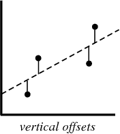
In the process of creating a regression model, all we try to do is draw a line as close to each point in the dataset as possible.
A typical example of this approach is the “least squares” linear regression approach, which calculates the closeness of a line in the up-to-down direction.
Example for illustration:
When you create a regression model, your end product is an equation by which you can predict the y values for the x value without knowing the y value in advance.
Logistic Regression
Logistic regression is similar to linear regression, except that instead of calculating the value of y, it evaluates which category a given data point belongs to.
What is Logistic Regression?
Logistic regression is a machine learning model used to solve classification problems.
Below are some examples of the classification tasks of MO:
- Email spam (spam or not spam?)
- Car insurance claim (compensation or repair?)
- Diagnostics of diseases
Each of these tasks has clearly 2 categories, making them examples of binary classification tasks.
Logistic regression works well for binary classification problems — we simply assign different categories to 0 and 1, respectively.
Why Logistic Regression? Because you cannot use linear regression for binary classification predictions. It simply won't work as you will be trying to draw a straight line through a dataset with two possible values.
This image can help you understand why linear regression is bad for binary classification:
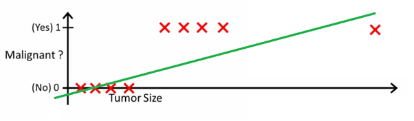
In this image, the y-axis represents the probability that the tumor is malignant. The 1-y values represent the probability that the tumor is benign. As you can see, the linear regression model performs very poorly for predicting the likelihood for most of the observations in the dataset.
This is why the logistic regression model is useful. It has a bend towards the best fit line, which makes it much more suitable for predicting qualitative (categorical) data.
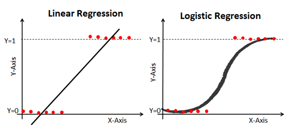
Here's an example that compares linear and logistic regression models on the same data:
Sigmoid (The Sigmoid Function)
The reason logistic regression is kinked is because it does not use a linear equation to calculate it. Instead, the logistic regression model is built using a sigmoid (also called a logistic function because it is used in logistic regression).
You don't have to memorize the sigmoid thoroughly to succeed in ML. Still, it will be helpful to have some idea of this feature.
Sigmoid Formula: The
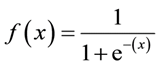
main characteristic of a sigmoid, which is worth dealing with - no matter what value you pass to this function, it will always return a value in the range 0-1.
Using a logistic regression model for predictions
In order to use logistic regression for predictions, you usually need to accurately define the cutoff point. This cut-off point is usually 0.5.
Let's use our cancer diagnosis example from the previous graph to see this principle in practice. If the logistic regression model returns a value below 0.5, then that data point will be categorized as benign. Similarly, if the sigmoid gives a value above 0.5, then the tumor is classified as malignant.
Using an error matrix to measure the effectiveness of logistic regression
The error matrix can be used as a tool to compare true positive, true negative, false positive, and false negative scores in MO.
The error matrix is particularly useful when used to measure the performance of a logistic regression model. Here is an example of how we can use the error matrix:
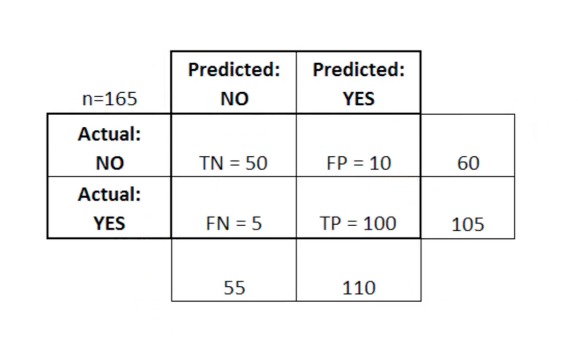
In this table TN stands for true negative, FN stands for false negative, FP stands for false positive, TP stands for true positive.
An error matrix is useful for evaluating a model if there are “weak” quadrants in the error matrix. As an example, she may have an abnormally high number of false positives.
It is also quite useful in some cases to ensure that your model is performing correctly in a particularly dangerous area of the error matrix.
In this example of a cancer diagnosis, for example, you would like to make sure that your model does not have too many false positives because this will mean that you diagnosed someone's malignant tumor as benign.
Summarize
In this section, you had your first acquaintance with the ML model - logistic regression.
Here's a quick summary of what you've learned about logistic regression:
- Types of classification problems that are suitable for solving with logistic regression
- Logistic function (sigmoid) always gives a value between 0 and 1
- How to use cut-off points to predict with a logistic regression model
- Why is an error matrix useful for measuring the performance of a logistic regression model
K-Nearest Neighbors Algorithm
The k-nearest neighbors algorithm can help solve the classification problem in the case when there are more than 2 categories.
What is the k-nearest neighbors algorithm?
This is a classification algorithm based on a simple principle. In fact, the principle is so simple that it is best to demonstrate it with an example.
Imagine you have height and weight data for footballers and basketball players. The k-nearest neighbors algorithm can be used to predict whether a new player is a soccer player or a basketball player. To do this, the algorithm determines the K data points closest to the study object.
This image demonstrates this principle with the parameter K = 3:
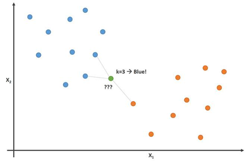
In this image, soccer players are blue and basketball players are orange. The point we are trying to classify is colored green. Since most (2 of 3) marks closest to the green point are colored blue (football players), the K-nearest neighbors algorithm predicts that the new player will also be a football player.
How to build a K-nearest neighbors algorithm
The main steps for building this algorithm:
- Collect all data
- Calculate the Euclidean distance from the new data point x to all other points in the data set
- Sort points from dataset in ascending order of distance to x
- Predict the answer using the same category as most of the K-closest data to x
Importance of the K variable in the K-nearest neighbors algorithm
While this may not be obvious from the outset, changing the K value in this algorithm will change the category that the new data point falls into.
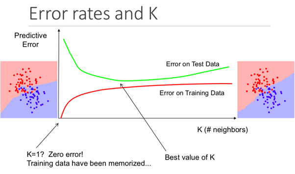
More specifically, too low a K value will cause your model to predict accurately on the training dataset, but be extremely ineffective on the test data. Also, having too high a K will make the model unnecessarily complex.
The illustration below shows this effect perfectly:
Pros and cons of the K-nearest neighbors algorithm
To summarize our introduction to this algorithm, let's briefly discuss the pros and cons of using it.
Pros:
- The algorithm is simple and easy to understand
- Trivial model training on new training data
- Works with any number of categories in a classification task
- Easily add more data to lots of data
- The model only takes 2 parameters: K and the distance metric you would like to use (usually Euclidean distance)
Minuses:
- High computation cost, because you need to process the entire amount of data
- Doesn't work as well with categorical parameters
Summarize
A summary of what you just learned about the K-Nearest Neighbor Algorithm:
- An example of a classification problem (football or basketball players) that the algorithm can solve
- How the algorithm uses Euclidean distance to neighboring points to predict which category a new data point belongs to
- Why K values are important for forecasting
- Pros and cons of using the K-nearest neighbors algorithm
Decision Trees and Random Forests
Decision tree and random forest are 2 examples of a tree method. More precisely, decision trees are ML models used to predict by looping through each function in a dataset one by one. A random forest is an ensemble (committee) of decision trees that use random orders of objects in a dataset.
What is a tree method?
Before we dive into the theoretical foundations of the tree-based method in ML, it is helpful to start with an example.
Imagine you are playing basketball every Monday. Moreover, you always invite the same friend to come and play with you. Sometimes a friend does come, sometimes not. The decision to come or not depends on many factors: what kind of weather, temperature, wind and fatigue. You start to notice these features and track them along with your friend's decision to play or not.
You can use this data to predict if your friend is coming today or not. One technique you can use is a decision tree. This is how it looks:
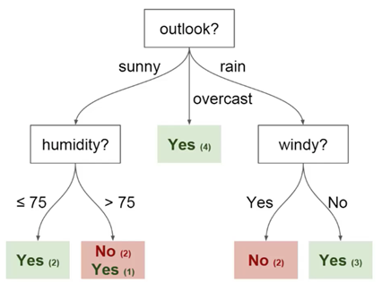
Each decision tree has 2 types of elements:
- Nodes: places where the tree is split based on the value of a certain parameter
- Edges: the result of the split leading to the next node
You can see that the diagram has nodes for outlook, humidity and
windy. And also the facets for each potential value of each of these parameters.
Here are a couple more definitions that you should understand before we start:
- Root - the node from which the division of the tree begins
- Leaves - the final nodes that predict the final result
You now have a basic understanding of what a decision tree is. We'll look at how to build such a tree from scratch in the next section.
How to build a decision tree from scratch
Building a decision tree is trickier than it sounds. This is because deciding which ramifications (characteristics) to divide your data into (which is a topic from entropy and data acquisition) is a mathematically challenging task.
To solve this problem, ML specialists usually use many decision trees, applying random sets of characteristics chosen to divide the tree into them. In other words, new random sets of characteristics are chosen for each separate tree, at each separate partition. This technique is called random forests.
In general, experts usually choose the size of a random set of features (denoted by m) so that it is the square root of the total number of features in the dataset (denoted by p). In short, m is the square root of p, and then a specific characteristic is randomly selected from m.
Benefits of using a random forest
Imagine that you are working with a lot of data that has one "strong" characteristic. In other words, there is a characteristic in this dataset that is much more predictable in terms of the end result than other characteristics of this dataset.
If you are building a decision tree by hand, then it makes sense to use this characteristic for the “top” partition in your tree. This means that you will have several trees whose predictions are highly correlated.
We want to avoid this because using the mean of highly correlated variables does not significantly reduce variance. By using random sets of characteristics for each tree in a random forest, we decorrelate the trees and the variance of the resulting model decreases. This decorrelation is a major advantage in using random forests over hand-built decision trees.
Summarize
So here's a quick summary of what you just learned about decision trees and random forests:
- An example of a problem whose solution can be predicted using a decision tree
- Decision tree elements: nodes, faces, roots, and leaves
- How using a random set of characteristics allows us to build a random forest
- Why using a random forest for decorrelation of variables can be useful in reducing the variance of the resulting model
Support Vector Machines
Support vector machines are a classification algorithm (although, technically speaking, they can also be used to solve regression problems) that divides a set of data into categories at the largest "gaps" between categories. This concept becomes clearer when you look at the following example.
What is support vector machine?
A support vector machine (SVM) is a supervised ML model with appropriate learning algorithms that analyze data and recognize patterns. The SVM can be used for both classification tasks and regression analysis. In this article, we will look specifically at using support vector machines to solve classification problems.
How does the MOU work?
Let's take a deeper dive into how the MOU really works.
We are given a set of training examples, each of which is marked as belonging to one of 2 categories, and using this set of SVMs we build a model. This model categorizes new examples into one of two categories. This makes the SVM an improbable binary linear classifier.
The MOU uses geometry to make predictions by category. More specifically, the support vector machine maps data points as points in space and categorizes them so that they are separated by as wide a gap as possible. The prediction that new data points will belong to a particular category is based on which side of the break point is.
Here is a visualization example to help you understand the intuition of the MOU:
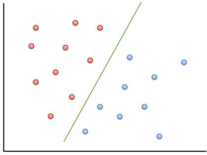
As you can observe, if a new data point falls to the left of the green line, it will be referred to as “red”, and if to the right, it will be referred to as “blue”. This green line is called a hyperplane and is an important term for working with MOUs.
Let's take a look at the following visual representation of the SVM:
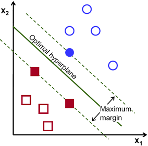
In this diagram, the hyperplane is labeled as the "optimal hyperplane". Support Vector Machine theory defines an optimal hyperplane as a hyperplane that maximizes the field between the two nearest data points from different categories.
As you can see, the field boundary does indeed affect 3 data points - 2 from the red category and 1 from the blue. These points, which are in contact with the border of the field, are called support vectors - hence the name.
Summarize
Here's a quick snapshot of what you just learned about support vector machines:
- The MOU is an example of a supervised ML algorithm
- The support vector can be used to solve both classification problems and for regression analysis.
- How the MOU categorizes data using a hyperplane that maximizes the margin between categories in the dataset
- That data points that touch the boundaries of the dividing field are called support vectors. This is where the name of the method comes from.
K-Means Clustering
The K-Means Method is an unsupervised machine learning algorithm. This means that it accepts untagged data and tries to cluster clusters of similar observations in your data. The K-Means method is extremely useful for solving real-world applications. Here are examples of several tasks that fit this model:
- Customer segmentation for marketing teams
- Classification of documents
- Optimizing shipping routes for companies like Amazon, UPS or FedEx
- Identifying and responding to criminal locations in the city
- Professional sports analytics
- Predicting and preventing cybercrime
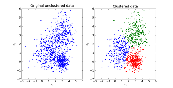
The main goal of the K-Means method is to divide the data set into distinguishable groups so that the elements within each group are similar to each other.
Here is a visual representation of what it looks like in practice:
We will explore the mathematics behind the K-Means method in the next section of this article.
How does the K-Means method work?
The first step in using the K-Means method is to choose the number of groups into which you want to divide your data. This quantity is the value of K, reflected in the name of the algorithm. The choice of the K value in the K-Means method is very important. We'll discuss how to choose the correct K value a little later.
Next, you must randomly select a point in the dataset and assign it to a random cluster. This will give you the starting data position at which you run the next iteration until the clusters stop changing:
- Calculating the centroid (center of gravity) of each cluster by taking the mean vector of points in that cluster
- Reassign each data point to the cluster whose centroid is closest to the point
Choosing an Appropriate K-value in the K-Means Method
Strictly speaking, choosing a suitable K value is quite difficult. There is no “right” answer in choosing the “best” K value. One method that ML professionals often use is called the “elbow method”.
To use this method, the first thing you need to do is calculate the sum of squared errors - the standard deviation for your algorithm for a group of K values. The standard deviation in the K-means method is defined as the sum of the squared distances between each data point in the cluster. and the center of gravity of this cluster.
As an example of this step, you can calculate the standard deviation for the K values of 2, 4, 6, 8, and 10. Next, you will want to generate a graph of the standard deviation and these K values. You will see that the deviation decreases as the K value increases.
And it makes sense: the more categories you create from a set of data, the more likely each data point will be close to the center of that point's cluster.
With that said, the main idea behind the elbow method is to choose the K value at which the RMS will dramatically slow down the rate of decline. This sharp decline forms an “elbow” on the chart.
As an example, here is a plot of RMS versus K. In this case, the elbow method will suggest using a K value of about 6.
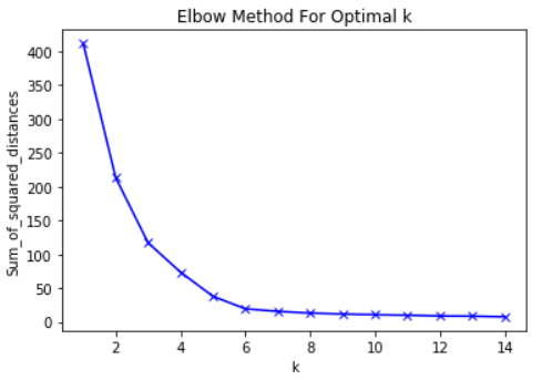
It is important that K = 6 is simply an estimate of an acceptable K value. There is no "best" K value in the K-Means method. Like many things in ML, this is a very situational decision.
Summarize
Here's a quick sketch of what you've just learned in this section:
- Examples of ML tasks without a teacher that can be solved by the K-means method
- Basic principles of the K-means method
- How K-Means Works
- How to use the elbow method to select the appropriate value for the K parameter in this algorithm
Principal Component Analysis
Principal component analysis is used to transform a dataset with many parameters into a new dataset with fewer parameters, and each new parameter in this dataset is a linear combination of previously existing parameters. This transformed data tends to justify much of the variance of the original dataset with much more simplicity.
What is Principal Component Method?
Principal component analysis (PCA) is an ML technique that is used to study the relationships between sets of variables. In other words, the PCA examines sets of variables in order to determine the basic structure of these variables. PCA is also sometimes called factor analysis.
Based on this description, you might think that PCA is very similar to linear regression. But this is not the case. In fact, these 2 techniques have several important differences.
Differences between linear regression and PCA
Linear regression determines the line of best fit across the dataset. Principal component analysis identifies multiple orthogonal best-fit lines for a dataset.
If you are not familiar with the term orthogonal, then it simply means that the lines are at right angles to each other, like north, east, south and west on a map.
Let's look at an example to help you understand this better.

Take a look at the axis labels in this image. The main component of the x-axis explains 73% of the variance in this dataset. The major component of the y-axis explains about 23% of the variance in the dataset.
This means that 4% of the variance remains unexplained. You can reduce this number by adding more principal components to your analysis.
Summarize
A summary of what you just learned about principal component analysis:
- PCA tries to find orthogonal factors that determine variability in a dataset
- Difference between linear regression and PCA
- What orthogonal principal components look like when rendered in a dataset
- That adding additional principal components can help explain variance more accurately in the dataset