MLflow in the cloud. A quick and easy way to bring ML models into production

Robot factory by lucart



MLflow is one of the most stable and lightweight tools to enable Data Scientists to manage the lifecycle of machine learning models. It is a user-friendly tool with a simple interface for viewing experiments and powerful tools for packaging management, deploying models. It allows you to work with almost any machine learning library.



I am Alexander Volynsky, architect of the cloud platform Mail.ru Cloud Solutions. In the last article, we covered Kubeflow. MLflow is another tool for building MLOps that does not require Kubernetes to work with.



I talked about MLOps in detail in the last article, now I will only briefly mention the main theses.

• MLOps stands for Machine Learning DevOps.
• Helps to standardize the machine learning model development process.
• Reduces the time it takes to roll out models into production.
• Includes tasks for tracking models, versioning and monitoring.

All this allows the business to get more value from machine learning models.



So, in the course of this article, we:

1. We will deploy services in the cloud that act as a backend for MLflow.
2. Install and configure MLflow Tracking Server.
3. Let's deploy JupyterHub and configure it to work with MLflow.
4. We will test manual and automatic logging of parameters and metrics of experiments.
5. Let's try different ways of publishing models.

It is important that we do this as close as possible to the production version. Most of the instructions on the Internet suggest deploying MLflow on a local machine or from a docker image. These options are fine for familiarization and quick experimentation, but not for production. We will use reliable cloud services.

If you prefer video tutorials , you can watch the webinar “ MLflow in the Cloud. A simple and quick way to bring ML models into production . "

MLflow: purpose and main components

MLflow is an open source platform for lifecycle management of machine learning models. It also solves the problems of reproducing experiments, publishing models, and includes a central register of models.



Unlike Kubeflow, MLflow can run without Kubernetes. But at the same time, MLflow knows how to package models into Docker images so that they can then be deployed to Kubernetes.



MLflow consists of several components.



MLflow Tracking... This is a convenient UI where you can view artifacts: graphs, sample data, datasets. You can also view the metrics and parameters of the models. MLflow Tracking has an API for different programming languages ​​with which you can log metrics, parameters and artifacts. Python, Java, R, REST are supported.



There are two important concepts in MLflow Tracking: runs and experiments.

• Run is a single iteration of the experiment. For example, you set the parameters of the model and run it for training. For this single launch, a new entry will appear in MLflow Tracking. When the model parameters change, a new run will be created.
• Experiment allows you to group multiple Runs into one entity so that you can easily view them.

You can deploy MLflow Tracking in various scenarios. We will use the option closest to production - scenario # 4 (as it is called in the official MLflow documentation ).





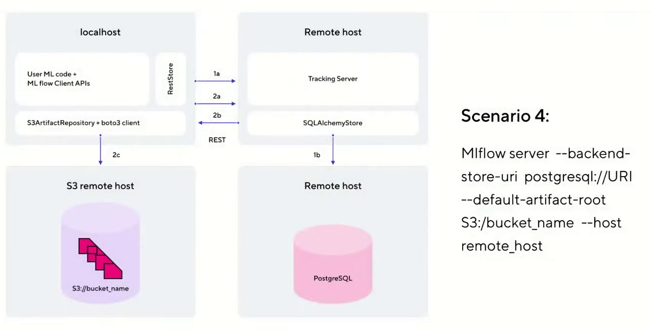
This option has a host on which JupyterHub is deployed. It communicates with the Tracking Server hosted on a separate virtual machine in the cloud. To store metadata about experiments, PostgreSQL is used, which we will deploy as a service in the cloud. And all artifacts and models are stored separately in S3 Object Storage.



MLflow Models . This component is responsible for packaging, storing and publishing models. It represents the concept of flavor. This is a kind of wrapper that allows you to use the model in various tools and frameworks without the need for additional integrations. For example, you can use models from Scikit-learn, Keras, TenserFlow, Spark MLlib, and other frameworks.



MLflow Models also allows you to make models available via the REST API and package them into a Docker image for later use in Kubernetes.



MLflow Registry . This component is the central repository of models. It includes a UI that allows you to add tags and descriptions for each model. It also allows you to compare different models with each other, for example, to see the differences in parameters.



MLflow Registry manages the life cycle of a model. In the context of MLflow, there are three lifecycle stages: Staging, Production, and Archived. There is also support for versioning. All this allows you to conveniently manage the entire rollout of models.



MLflow Projects... It's a way to organize and describe your code. Each project is a directory with a set of files, most often these are pipelines. Each project is described by a separate MLProject file in yaml format. It specifies the project name, environment and entrypoints. This allows the experiment to be reproduced in a different environment. There is also a CLI and API for Python.



With MLflow Projects, you can create modules that are reusable steps. These modules can then be embedded in more complex pipelines, allowing them to be standardized.

Instructions for installing and configuring MLflow

Step 1: deploy services in the cloud that act as a backend

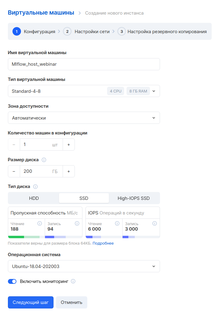
First, we will create a virtual machine on which we will deploy MLflow Tracking Server. We will do this on our cloud platform Mail.ru Cloud Solutions (new users here receive 3000 bonus rubles for testing, so you can register and repeat everything described here). 

Before starting work, you need to configure the network, generate and download an SSH key to connect to the virtual machine. You can configure the network yourself according to the instructions .

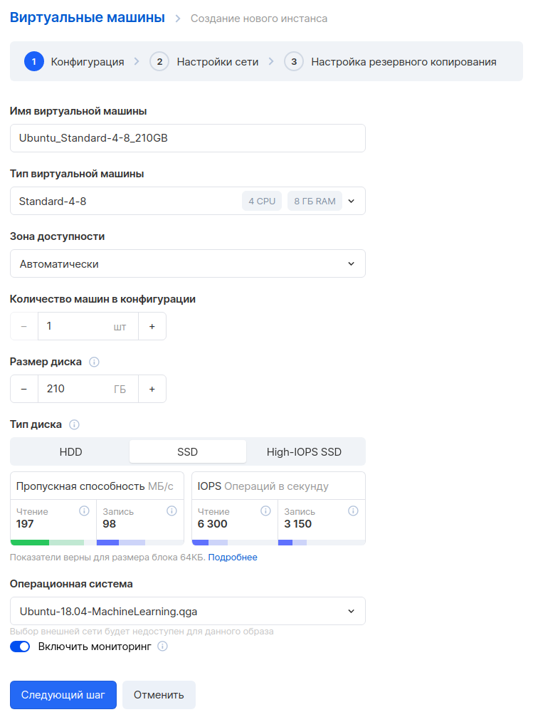
Go to the MCS panel, section " Cloud Computing - Virtual Machines ", and click the "Add" button. Next, we set the parameters of the new virtual machine. For example, we will take a configuration with 4 CPUs and 8 GB of RAM. Let's choose the OS - Ubuntu 18.04.





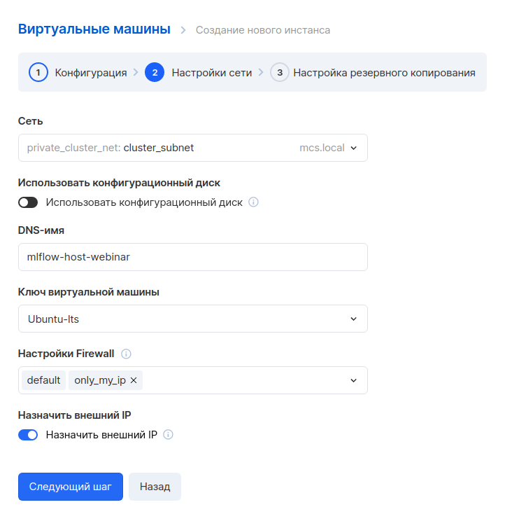
The next step is to configure the network. Since we have already created a network in advance, here you just need to select it. Please note that a custom rule is specified in the Firewall settings - only_my_ip. This rule is absent by default, we created it ourselves so that you can connect to a virtual machine only from a specific address. We recommend that you do the same to improve security. Here's how to create your own rules.



You also need to assign an external IP so that you can connect to the machine from the Internet.





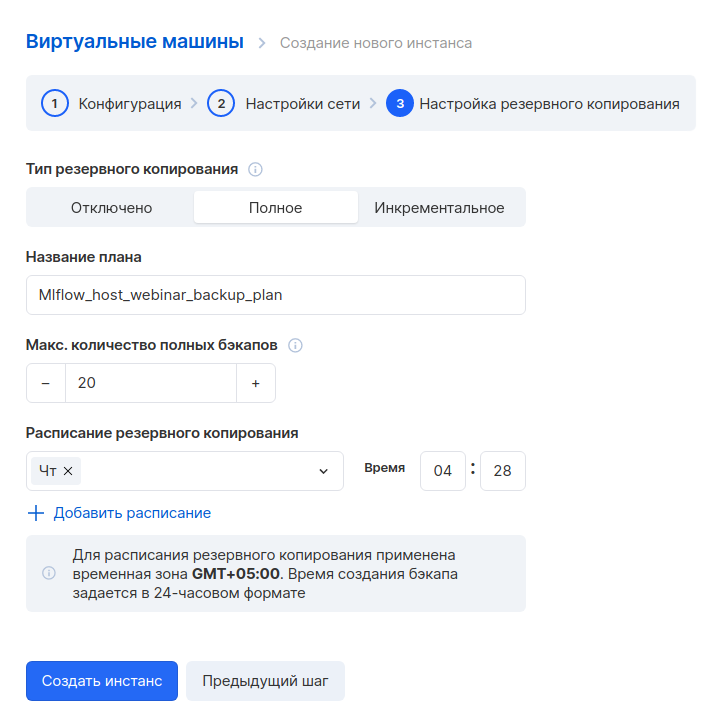
In the next step, we set up a backup. You can leave the default settings if you like.





We create an instance and wait a few minutes. When the virtual machine is ready, you will need to write down its internal and external addresses, they will be useful later.





Next, let's create a database. Go to the " Databases " section and click the "Add" button. We select PostgreSQL 12 in the Master-slave configuration.





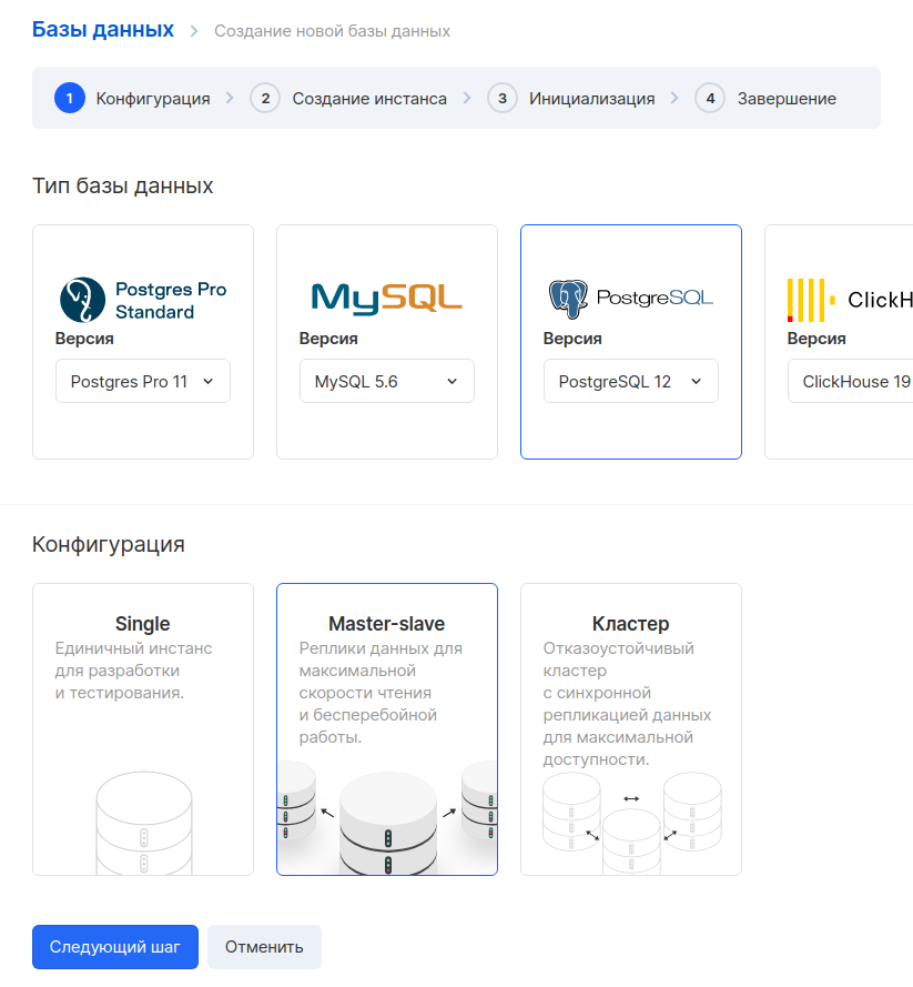
In the next step, we set the parameters of the virtual machine. As an example, we took a configuration with 1 CPU and 2 GB of RAM. The external IP can be omitted, because we will only access this machine from the internal network. It is important to select the same network that we chose for the Tracking Server VM.





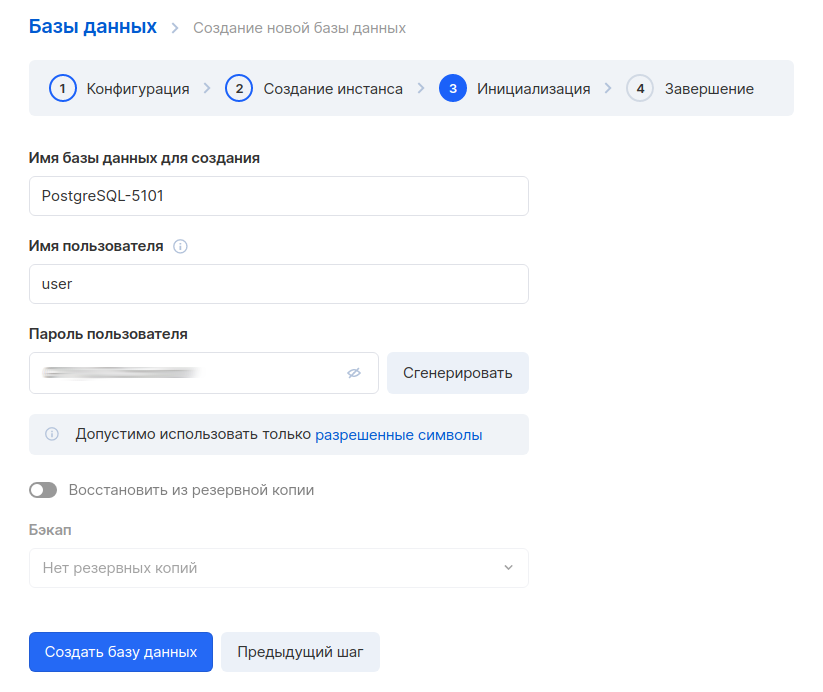
The next step is to generate a database name, user and password. It is good practice to create a separate database and a separate user for each service.





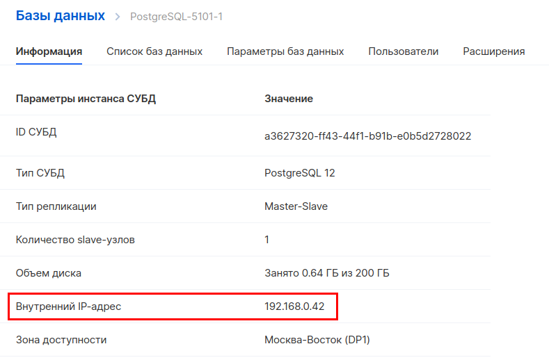
After creating the database, you also need to write down the internal address. You will need it to set up a connection to MLflow.





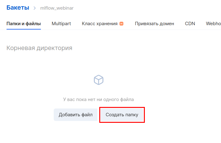
Next, you need to create a new bucket in object storage. Go to the " Object Storage - Buckets " section and create a new bucket. When creating, specify the name and type - Hotbox.





Create a directory inside the bucket. To do this, go into it and click "Create folder". By default, the MLflow instruction uses the name of the artifacts folder, so we will use the same name.





Next, you need to create a separate account to access this bucket. In the "Object storage" section, go to the " Accounts " subsection and click "Add account".





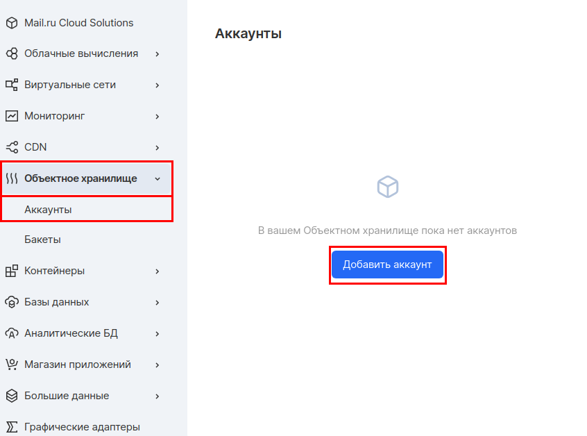
We will use the account name - mlflow_webinar. After creation, write down the Access Key ID and Secret Key. The Secret Key is especially important, because it will no longer be visible, and in case of loss, you will have to recreate it.





That's it, we have prepared the infrastructure for the backend.



All services are in one virtual network. Therefore, for communication between them, we will use internal addresses everywhere. If you want to use external addresses, you need to configure the Firewall correctly.

Step 2: install and configure MLflow Tracking Server on a dedicated VM

We connect via SSH to the virtual machine that we created at the very beginning. Here's how to do it.



First, install conda , which is a package manager for Python, R and other languages.

curl -O https://repo.anaconda.com/archive/Anaconda3-2020.11-Linux-x86_64.sh
bash Anaconda3-2020.11-Linux-x86_64.sh
exec bash
      
      

        
        
        
      

    
        
        
        
      
      

        
        
        
      

    
    

Next, let's create and activate a separate environment for MLflow.

conda create -n mlflow_env
conda activate mlflow_env
      
      

        
        
        
      

    
        
        
        
      
      

        
        
        
      

    
    

Install the required libraries:

conda install python
pip install mlflow
pip install boto3
sudo apt install gcc
pip install psycopg2-binary
      
      

        
        
        
      

    
        
        
        
      
      

        
        
        
      

    
    

Next, you need to create environment variables to access S3. Open the file for editing:

sudo nano /etc/environment
      
      

        
        
        
      

    
        
        
        
      
      

        
        
        
      

    
    

And we set variables in it. Instead of REPLACE_WITH_INTERNAL_IP_MLFLOW_VM, you need to substitute the address of your virtual machine:

MLFLOW_S3_ENDPOINT_URL=https://hb.bizmrg.com
MLFLOW_TRACKING_URI=http://REPLACE_WITH_INTERNAL_IP_MLFLOW_VM:8000
      
      

        
        
        
      

    
        
        
        
      
      

        
        
        
      

    
    

MLflow communicates with S3 using the boto3 library, which by default looks for credentials in the ~ / .aws folder. Therefore, we need to create a file:

mkdir ~/.aws
nano ~/.aws/credentials
      
      

        
        
        
      

    
        
        
        
      
      

        
        
        
      

    
    

In this file we will write the credentials for access to S3, which we received after creating the bucket:

[default]
aws_access_key_id = REPLACE_WITH_YOUR_KEY
aws_secret_access_key = REPLACE_WITH_YOUR_SECRET_KEY
      
      

        
        
        
      

    
        
        
        
      
      

        
        
        
      

    
    

Finally, we apply the environment settings:

conda activate mlflow_env
      
      

        
        
        
      

    
        
        
        
      
      

        
        
        
      

    
    

Now you can start Tracking Server. Substitute your PostgreSQL and S3 connection parameters into the command:

mlflow server --backend-store-uri postgresql://pg_user:pg_password@REPLACE_WITH_INTERNAL_IP_POSTGRESQL/db_name --default-artifact-root s3://REPLACE_WITH_YOUR_BUCKET/REPLACE_WITH_YOUR_DIRECTORY/ -h 0.0.0.0 -p 8000

      
      

        
        
        
      

    
        
        
        
      
      

        
        
        
      

    
    

MLflow launched:





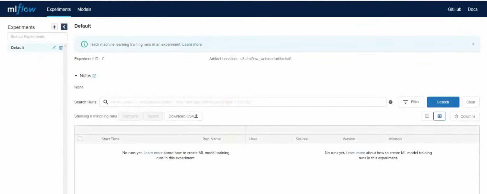
Now let's open the GUI and check that everything works as it should. To do this, you need to go to the external IP address of the virtual machine with MLflow Tracking Server, port 8000. In our case, it will be 37.139.41.57 : 8000





MLflow started



But now there is a small problem in our schema. The server works as long as the terminal is running. If you close the terminal, MLflow will stop. Also it won't restart automatically if we restart the server. To fix this, we will start the MLflow server as a systemd service.



So, let's create two directories for storing logs and errors:

mkdir ~/mlflow_logs/
mkdir ~/mlflow_errors/
      
      

        
        
        
      

    
        
        
        
      
      

        
        
        
      

    
    

Next, let's create a service file:

sudo nano /etc/systemd/system/mlflow-tracking.service

      
      

        
        
        
      

    
        
        
        
      
      

        
        
        
      

    
    

Next, add the code to it. Do not forget to substitute your parameters for connecting to the database and S3, as you did when starting the server manually:

[Unit]
Description=MLflow Tracking Server
After=network.target

[Service]
Environment=MLFLOW_S3_ENDPOINT_URL=https://hb.bizmrg.com
Restart=on-failure
RestartSec=30
StandardOutput=file:/home/ubuntu/mlflow_logs/stdout.log
StandardError=file:/home/ubuntu/mlflow_errors/stderr.log
User=ubuntu
ExecStart=/bin/bash -c 'PATH=/home/ubuntu/anaconda3/envs/mlflow_env/bin/:$PATH exec mlflow server --backend-store-uri postgresql://PG_USER:PG_PASSWORD@REPLACE_WITH_INTERNAL_IP_POSTGRESQL/DB_NAME --default-artifact-root s3://REPLACE_WITH_YOUR_BUCKET/REPLACE_WITH_YOUR_DIRECTORY/ -h 0.0.0.0 -p 8000' 

[Install]
WantedBy=multi-user.target
      
      

        
        
        
      

    
        
        
        
      
      

        
        
        
      

    
    

Now we start the service, activate autoload at system startup and check that the service is running:

sudo systemctl daemon-reload
sudo systemctl enable mlflow-tracking
sudo systemctl start mlflow-tracking
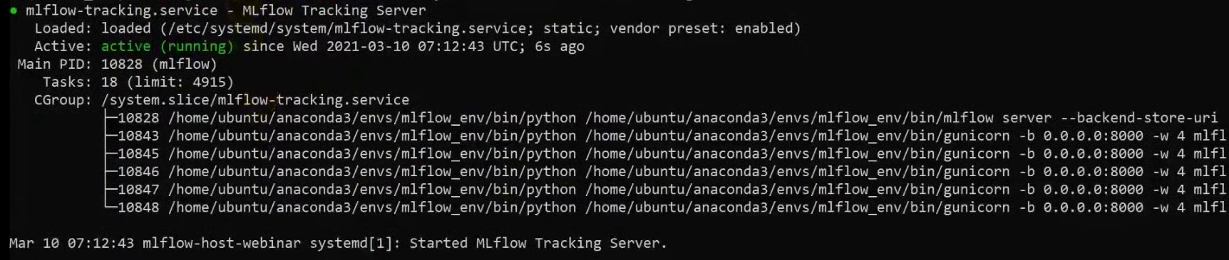
sudo systemctl status mlflow-tracking
      
      

        
        
        
      

    
        
        
        
      
      

        
        
        
      

    
    

We see that the service has started:





In addition, we can check the logs, everything is fine there too:

head -n 95 ~/mlflow_logs/stdout.log

      
      

        
        
        
      

    
        
        
        
      
      

        
        
        
      

    
    

Open the web interface again and see that the MLflow server is running. That's it, MLflow Tracking Server is installed and ready to go.

Step 3: deploy JupyterHub in the cloud and configure it to work with MLflow

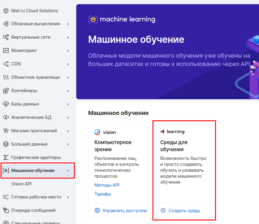
We will deploy JupyterHub on a separate virtual machine so that later this host can be provided to teams of data engineers or data scientists. This way they can work with JupyterHub, but they cannot affect the MLflow server. We'll use our Machine Learning in the Cloud service, which allows you to quickly get a ready-to-go environment with JupyterHub, conda and other useful tools installed.



In the MCS panel, go to the Machine Learning section and create a learning environment.





We select the parameters of the virtual machine. We'll take 4 CPUs and 8 GB of RAM.





In the next step, we set up the network. Make sure the network is the same so that this machine can communicate with the rest of the servers on the internal network. Select the "Assign external IP" option so that later we can connect to this machine from the Internet.





The last step is to set up your backup. You can leave the default options.



After the virtual machine is created, you need to write down its external IP address: it will be useful to us later.





Now we connect to this machine via SSH and activate the installed JupyterHub. We'll be using the tmux utility so that we can detach from the screen and run other commands.

tmux
jupyter-notebook --ip '*'
      
      

        
        
        
      

    
        
        
        
      
      

        
        
        
      

    
    

Using tmux is not a product solution. Now we will do this as part of a test project, and for product solutions we recommend using systemd, as we did to launch MLflow Tracking Server.



After activating JupyterHub, the console will have a URL where you need to go and log in to JupyterHub. In this line, you must substitute the external IP address of the virtual machine.





Go to this address and see the JupyterHub interface:





Now we need to leave the server running, but at the same time execute other commands. Therefore, we will disconnect from this terminal instance and leave it running in the background. To do this, press the key combination ctrl + b d.



Direct loading of artifacts into artefact storage will be performed from this host. Therefore, we need to set up JupyterHub interoperability with both MLflow and S3. First, let's set up a few environment variables. Let's open the / etc / environment file:

sudo nano /etc/environment
      
      

        
        
        
      

    
        
        
        
      
      

        
        
        
      

    
    

And write the Tracking Server and Endpoint addresses for S3 into it:

MLFLOW_TRACKING_URI=http://REPLACE_WITH_INTERNAL_IP_MLFLOW_VM:8000
MLFLOW_S3_ENDPOINT_URL=https://hb.bizmrg.com
      
      

        
        
        
      

    
        
        
        
      
      

        
        
        
      

    
    

We also need to re-create the credentials to access S3. Let's create a file and directory:

mkdir .aws
nano ~/.aws/credentials
      
      

        
        
        
      

    
        
        
        
      
      

        
        
        
      

    
    

Let's write the Access Key and Secret Key there:

[default]
aws_access_key_id = REPLACE_WITH_YOUR_KEY
aws_secret_access_key = REPLACE_WITH_YOUR_SECRET_KEY
      
      

        
        
        
      

    
        
        
        
      
      

        
        
        
      

    
    

Now let's install MLflow to use its client side. To do this, let's create a separate environment and a separate kernel:

conda create -n mlflow_env
conda activate mlflow_env
conda install python
pip install mlflow
pip install matplotlib
pip install sklearn
pip install boto3
conda install -c anaconda ipykernel
python -m ipykernel install --user --name ex --display-name "Python (mlflow)"
      
      

        
        
        
      

    
        
        
        
      
      

        
        
        
      

    
    

Step 4: log parameters and metrics of experiments

Now we will work directly with the code. Go to the JupyterHub web interface again, launch the terminal and clone the repository:

git clone https://github.com/stockblog/webinar_mlflow/ webinar_mlflow

      
      

        
        
        
      

    
        
        
        
      
      

        
        
        
      

    
    

Next, open the mlflow_demo.ipynb file and sequentially launch the cells.



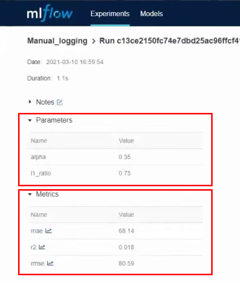
In cell number 3, we will test manual logging of parameters and metrics. The cell clearly indicates the parameters that we want to secure. We launch the cell and after it works, we go to the MLflow interface. Here we see that a new experiment has been created - Manual_logging.





We go into the details of this experiment and see the parameters and metrics that we specified during logging:





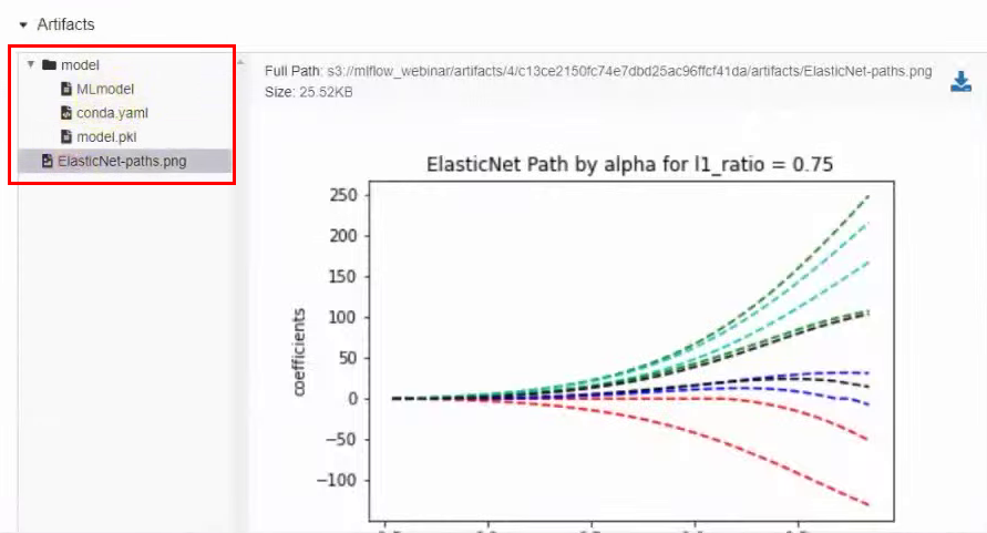
In the same window below there are artifacts that are directly related to the model, for example, a graph:





Now let's try to log all parameters automatically. In the next cell, we use the same model, but we turn on auto-logging. The line is responsible for this:

mlflow.sklearn.autolog(log_input_examples=True)

      
      

        
        
        
      

    
        
        
        
      
      

        
        
        
      

    
    

We need to specify the flavor that we will use, in our case it is sklearn. We also specified log_input_examples = True in the parameters of the autolog function. At the same time, examples of input data for the model will be automatically logged: which columns, what they mean and what the input data looks like. This information will be found in artifacts. This can come in handy when a team is working on multiple experiments at the same time. Because it is not always possible to keep in mind every model and all the data examples for it.



In this cell, we have removed all the lines associated with manual logging of metrics and parameters. But logging of artifacts remains in manual mode.



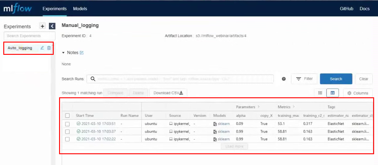
We launch the cell, after its execution, a new experiment is created. Go to the MLflow interface, go to the Auto_logging experiment and see that now there are many more parameters and metrics than with manual collection:





Now, if we change the parameters in the cell and run it again, lines with new launches will appear in experiments in MLflow. For example, we made three launches with different parameters:





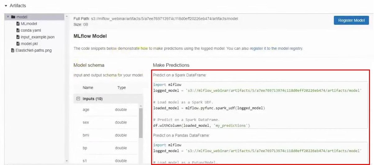
Also in the artifacts you can find an example of how to use this particular model. There is a model path in S3 and examples for different frameworks.

Step 5: Testing Ways to Publish ML Models

So, we did the experiments, and now we will publish the model. We'll look at two ways to do this.



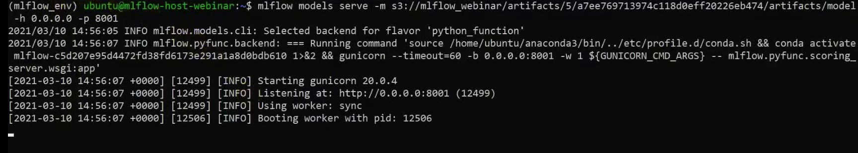
Publishing Method # 1: Access the S3 repository directly. Copy the address of the model to S3 storage and publish it using mlflow serve:

mlflow models serve -m s3://BUCKET/FOLDER/EXPERIMENT_NUMBER/INTERNAL_MLFLOW_ID/artifacts/model -h 0.0.0.0 -p 8001
      
      

        
        
        
      

    
        
        
        
      
      

        
        
        
      

    
    

In this command, we specify the host and port on which the model will be available. We use the address 0.0.0.0, which means the current host. There are no errors in the terminal, which means that the model has been published:





Now let's test it. In a new terminal window, connect via SSH to the same server and try to reach the model using curl. If you are using the same dataset, then you can completely copy the command without changes:

curl -X POST -H "Content-Type:application/json; format=pandas-split" --data '{"columns":["age", "sex", "bmi", "bp", "s1", "s2", "s3", "s4", "s5", "s6"], "data":[[0.0453409833354632, 0.0506801187398187, 0.0606183944448076, 0.0310533436263482, 0.0287020030602135, 0.0473467013092799, 0.0544457590642881, 0.0712099797536354, 0.133598980013008, 0.135611830689079]]}' http://0.0.0.0:8001/invocations
      
      

        
        
        
      

    
        
        
        
      
      

        
        
        
      

    
    

After executing the command, we see the result:





 

The model can also be accessed from the JupyterHub interface. To do this, run the appropriate cell , but before that, change the IP address to your own.



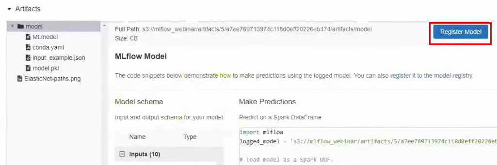
Publication method # 2: register the model in MLflow. We can also register the model in MLflow, and then it will be available through the UI interface. To do this, go back to the results of the experiment, in the Artifacts section, click the Register Model button and in the window that appears, give it a name.





Now in the top menu, go to the Models tab. And we see that in the list of models we have a new model:





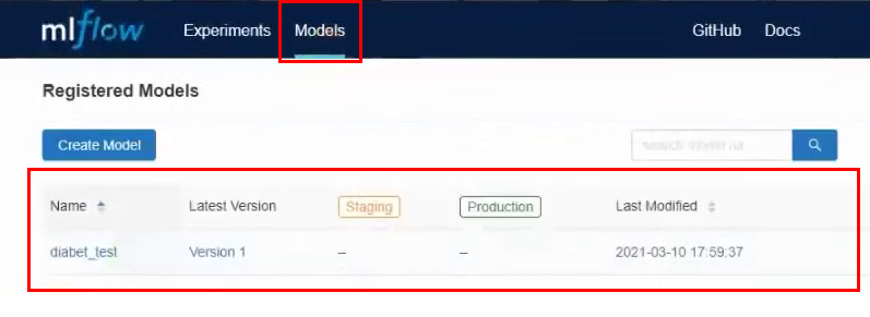
Let's go into it. In this interface, you can transfer the model to different stages, see the input parameters and results. You can also provide a description of the model, which will be useful if several people are working on it. We will convert our model to Staging.





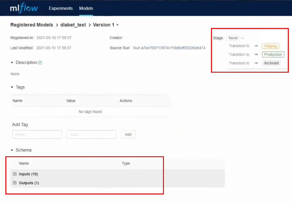
We do almost all actions through the interface, but in the same way you can work through the API and CLI. All these actions can be automated: registering models, transferring to another stage, rolling out models and everything else.



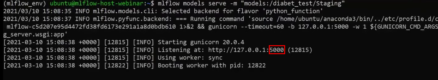
Now we'll also use the serve command to publish the model, but instead of the long path in S3, we'll just specify the name of the model:

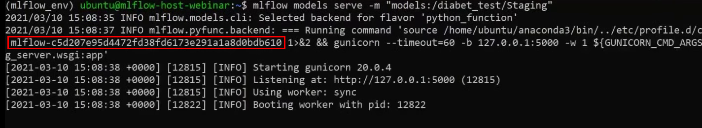
mlflow models serve -m "models:/YOUR_MODEL_NAME/STAGE"

      
      

        
        
        
      

    
        
        
        
      
      

        
        
        
      

    
    

Please note that this time we did not specify the port and the default model was published on port 5000:





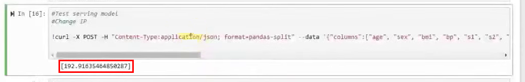
Now, using curl, we try to reach the model again:

curl -X POST -H "Content-Type:application/json; format=pandas-split" --data '{"columns":["age", "sex", "bmi", "bp", "s1", "s2", "s3", "s4", "s5", "s6"], "data":[[0.0453409833354632, 0.0506801187398187, 0.0606183944448076, 0.0310533436263482, 0.0287020030602135, 0.0473467013092799, 0.0544457590642881, 0.0712099797536354, 0.133598980013008, 0.135611830689079]]}' http://0.0.0.0:5000/invocations
      
      

        
        
        
      

    
        
        
        
      
      

        
        
        
      

    
    

The result is the same:





But if we try to access the model from another server, then we will fail. Because now the model is only available within the host where it is published. To fix this, let's publish the model with the -h parameter:

mlflow models serve -m "models:/YOUR_MODEL_NAME/STAGE" -h 0.0.0.0

      
      

        
        
        
      

    
        
        
        
      
      

        
        
        
      

    
    

Let's test access to the model using the same cell in the JupyterHub, but change the port to 5000. The model returns a result. It differs slightly from the result above, because during the webinar we changed some parameters.





The model can also be accessed using Python. An example can be found in another cell .



But there is a peculiarity in both versions of publishing the model. The model is available as long as the terminal is running with the serve command. When we close the terminal or restart the server, access to the model will be lost. To avoid this, we will publish the model using the systemd service, as we did to launch the MLflow Tracking Server.



Let's create a new service file:

sudo nano /etc/systemd/system/mlflow-model.service

      
      

        
        
        
      

    
        
        
        
      
      

        
        
        
      

    
    

And we will insert these commands into it, having previously replaced the variables with our own.

[Unit]
Description=MLFlow Model Serving
After=network.target

[Service]
Restart=on-failure
RestartSec=30
StandardOutput=file:/home/ubuntu/mlflow_logs/stdout.log
StandardError=file:/home/ubuntu/mlflow_errors/stderr.log
Environment=MLFLOW_TRACKING_URI=http://REPLACE_WITH_INTERNAL_IP_MLFLOW_VM:8000
Environment=MLFLOW_CONDA_HOME=/home/ubuntu/anaconda3/
Environment=MLFLOW_S3_ENDPOINT_URL=https://hb.bizmrg.com
ExecStart=/bin/bash -c 'PATH=/home/ubuntu/anaconda3/envs/REPLACE_WITH_MLFLOW_ENV_OF_MODEL/bin/:$PATH exec mlflow models serve -m "models:/YOUR_MODEL_NAME/STAGE" -h 0.0.0.0 -p 8001'

[Install]
WantedBy=multi-user.target
      
      

        
        
        
      

    
        
        
        
      
      

        
        
        
      

    
    

There is one new variable that we haven't used before: REPLACE_WITH_MLFLOW_ENV_OF_MODEL. This is an individual MLflow environment that is automatically created for each model. To see what environment your model is running in, look at the output of the serve command when you ran the model. There is this identifier in there:





Now let's start and activate this service so that the model is published every time the host starts:

sudo systemctl daemon-reload
sudo systemctl enable mlflow-model
sudo systemctl start mlflow-model
      
      

        
        
        
      

    
        
        
        
      
      

        
        
        
      

    
    

Checking the status:

sudo systemctl status mlflow-model

      
      

        
        
        
      

    
        
        
        
      
      

        
        
        
      

    
    

We see that an error appeared at startup:





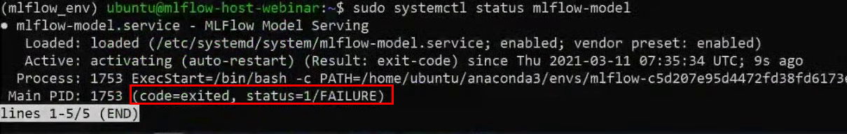
Using her example, we will analyze how you can find and eliminate errors. To understand what actually happened, let's check the logs. They are in a folder that we created specifically for logs.

head -n 95 ~/mlflow_logs/stdout.log

      
      

        
        
        
      

    
        
        
        
      
      

        
        
        
      

    
    

In our example, at the very end of the log, you can see that MLflow cannot find the boto3 library, which is required to access S3:





There are two options for how to solve the problem:

1. Install the library by hand into the MLflow environment. But this is a crutch method, we will not consider it.
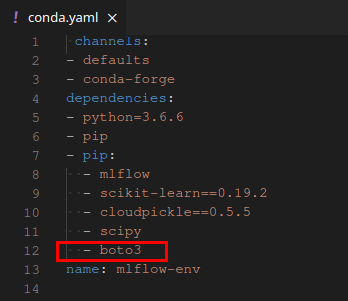
2. Register the library in dependencies in the yaml file. We will consider this method.

We need to find the folder in the bucket where this model is stored. To do this, go back to the MLflow interface and, in the experiment results, go to the section with artifacts. We remember the path:





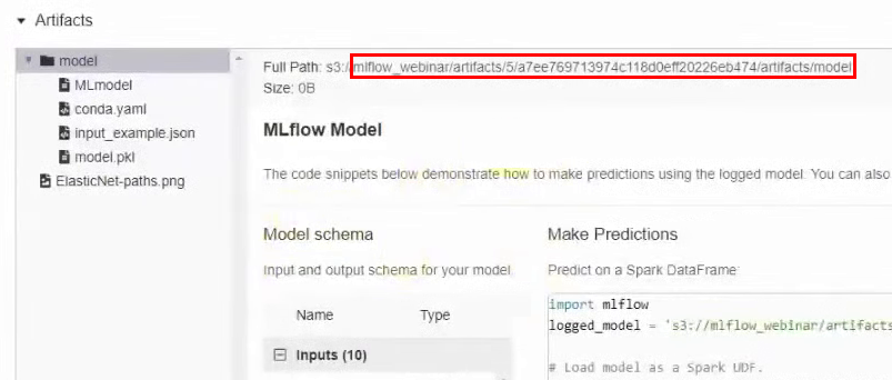
In the MCS interface, go to the bucket along this path and download the conda.yaml file.





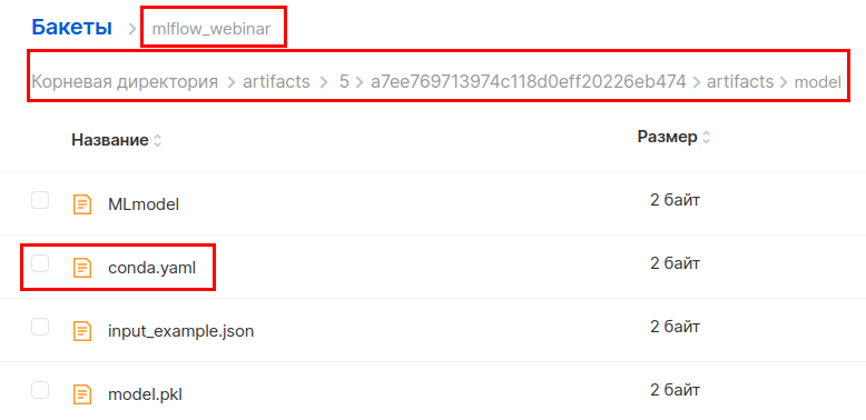
Add the boto3 library to the section with dependencies and upload the file back.





Let's try to start the systemd service again:

sudo systemctl start mlflow-model

      
      

        
        
        
      

    
        
        
        
      
      

        
        
        
      

    
    

Everything is fine now, the model has started. You can again try to reach her in different ways, as we did before. Note that the port should be specified again as 8001.



Now let's build a docker image with this model so that it can be easily migrated to another environment. To do this, docker must be installed on the host. We will not consider the installation process, but simply provide a link to the official instructions .



Let's execute the command:

mlflow models build-docker -m "models:/YOUR_MODEL_NAME/STAGE" -n "DOCKER_IMAGE_NAME"

      
      

        
        
        
      

    
        
        
        
      
      

        
        
        
      

    
    

In the -n parameter, we specify the desired name for the docker image. Result:





Let's test it. We launch the container, now the model will be available on port 5001:

docker run -p 5001:8080 YOUR_MODEL_NAME

      
      

        
        
        
      

    
        
        
        
      
      

        
        
        
      

    
    

The model should now be immediately available and active. Let's check:

curl -X POST -H "Content-Type:application/json; format=pandas-split" --data '{"columns":["age", "sex", "bmi", "bp", "s1", "s2", "s3", "s4", "s5", "s6"], "data":[[0.0453409833354632, 0.0506801187398187, 0.0606183944448076, 0.0310533436263482, 0.0287020030602135, 0.0473467013092799, 0.0544457590642881, 0.0712099797536354, 0.133598980013008, 0.135611830689079]]}' http://127.0.0.1:5001/invocations
      
      

        
        
        
      

    
        
        
        
      
      

        
        
        
      

    
    

You can also check availability from JupyterHub. At the same time, in the terminal where we launched the docker image, we see that requests come from two different hosts, local and JupyterHub:





That's it, the docker image is assembled, tested and ready to go.

What have we learned

So, we got acquainted with MLflow and learned how to deploy it in the cloud. Most of the instructions on the net are limited to installing MLflow on the local machine. This is good for familiarization and quick experimentation, but definitely not a production option.



All of this is possible because cloud platforms provide a variety of out-of-the-box services that help simplify and speed up deployment. 

, , Mail.ru Cloud Solutions, 3000 ₽. , MLflow .