The apparatus of linear algebra is used in various fields - in linear programming, econometrics, in the natural sciences. Separately, I note that this branch of mathematics is in demand in machine learning. If, for example, you need to work with matrices and vectors, then, quite possibly, at some step you will have to solve a system of linear algebraic equations (SLAE).
SLAE is a powerful process modeling tool. If some well-studied model based on SLAE is suitable for formalizing the problem, then it will be possible to solve it with a high probability. But how fast it depends on your tools and computing power.
I will tell you about one of such tools - the scipy.linalg Python package from the library SciPy , which allows you to quickly and efficiently solve many problems using the apparatus of linear algebra.
In this tutorial, you will learn:
- how to install scipy.linalg and prepare your code runtime;
- how to work with vectors and matrices using NumPy;
- why scipy.linalg is better than numpy.linalg;
- how to formalize problems using systems of linear algebraic equations;
- how to solve a SLAE using scipy.linalg ( with a real example).
If possible, do habraCUT here! It is important that people read this ^^ list and are interested.
When it comes to mathematics, the presentation of the material should be consistent - so that one follows from the other. This article is no exception: first there will be a lot of preparatory information and only then we will get down to business.
If you are ready for this, I invite you under cat. Although, to be honest, some sections can be skipped - for example, the basics of working with vectors and matrices in NumPy (if you are familiar with it).
Installing scipy.linalg
SciPy is an open source Python library for scientific computing: SLAE solution, optimization, integration, interpolation, and signal processing. Besides linalg, it contains several other packages - for example, NumPy, Matplotlib, SymPy, IPython, and pandas.
Among other things, scipy.linalg contains functions for working with matrices - calculating the determinant, inverse, calculating eigenvalues and vectors, and singular value decomposition.
To use scipy.linalg, you need to install and configure the SciPy library. This can be done using the Anaconda distribution and the Conda package management system and installer .
First, prepare the runtime for the library:
$ conda create --name linalg

$ conda activate linalg
Install the required packages:
(linalg) $ conda install scipy jupyter
This command can take a long time. Do not be alarmed!
I suggest using Jupyter Notebook to run your code in an interactive environment. This is not necessary, but for me personally, it makes my job easier.
Before opening the Jupyter Notebook, you need to register an instance of conda linalg to use as the kernel when creating the notebook. To do this, run the following command:
(linalg) $ python -m ipykernel install --user --name linalg
Now you can open Jupyter Notebook:
$ jupyter notebook
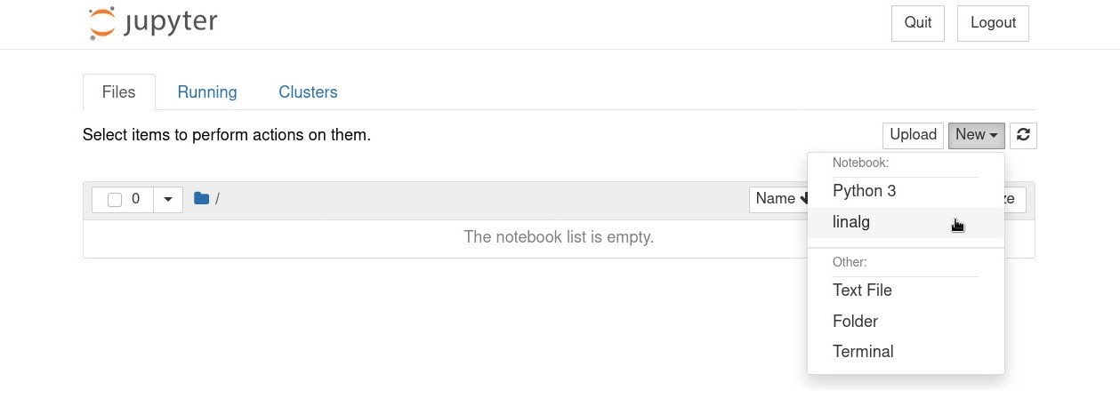
When it is loaded in your browser, create a new notebook, by clicking the New → linalg :
To verify that the SciPy library installation was successful, enter in your notebook:
>>>

In [1]: import scipy
NumPy for working with vectors and matrices (where without it)
It is difficult to overestimate the role of vectors and matrices in solving technical problems, including machine learning problems.
NumPy is the most popular package for working with matrices and vectors in Python. It is often used in conjunction with scipy.linalg. To get started with matrices and vectors, you need to import the NumPy package:
>>>

In [2]: import numpy as np
NumPy uses a special type called ndarray to represent matrices and vectors . To create an ndarray object, you can use array () .
For example, you need to create the following matrix:

Let's create a matrix as a set of nested lists (row vectors):
>>>

In [3]: A = np.array([[1, 2], [3, 4], [5, 6]])

   ...: A

Out[3]:

array([[1, 2],

       [3, 4],

       [5, 6]])
Note that the above output ( Outp [3] ) is a good enough representation of the resulting matrix.
And one more thing: all elements of the matrix must and will have the same type. This can be verified with dtype .
>>>

In [4]: A.dtype

Out[4]:

dtype('int64')
The elements here are integers, so their default generic type is int64 . If there was at least one floating point number among them, all elements would be float64 :
>>>

In [5]: A = np.array([[1.0, 2], [3, 4], [5, 6]])

   ...: A

Out[5]:

array([[1., 2.],

       [3., 4.],

       [5., 6.]])

In [6]: A.dtype

Out[6]:

dtype('float64')
To display the dimension of a matrix, you can use the shape method :
>>>

In [7]: A.shape

Out[7]:

(3, 2)
As expected, the dimension of the matrix A is 3 × 2, that is, A has three rows and two columns.
When working with matrices, you often need to use the transpose operation, which turns columns into rows and vice versa. To transpose a vector or matrix (represented by an object of type ndarray), you can use .transpose () or .T . For example:
>>>

In [8]: A.T

Out[8]:

array([[1., 3., 5.],

       [2., 4., 6.]])
You can also use .array () to create a vector, passing in a list of values as an argument:
>>>

In [9]: v = np.array([1, 2, 3])

   ...: v

Out[9]:

array([1, 2, 3])
Similar to matrices, we use .shape () to display the dimension of a vector:
>>>

In [10]: v.shape

Out[10]:

(3,)
Note that it looks like (3,), not like (3, 1) or (1, 3). The NumPy developers decided to make the vector dimension mapping the same as in MATLAB.
To get the dimension (1, 3) at the output, it would be necessary to create an array like this:
>>>

In [11]: v = np.array([[1, 2, 3]])

   ...: v.shape

Out[11]:

(1, 3)
For (3, 1) - like this:
>>>

In [12]: v = np.array([[1], [2], [3]])

   ...: v.shape

Out[12]:

(3, 1)
As you can see, they are not identical.
Often the problem arises from a row vector to make a column vector. Alternatively, you can first create a row vector and then use .reshape () to convert it to a column:
>>>

In [13]: v = np.array([1, 2, 3]).reshape(3, 1)

   ...: v.shape

Out[13]:

(3, 1)
In the above example, we used .reshape () to get a column vector of dimension (3, 1) from a vector of dimension (3,). It is worth noting that .reshape () does the transformation taking into account the fact that the number of elements (100% of filled places) in the array with the new dimension must be equal to the number of elements in the original array.
In practical tasks, it is often required to create matrices entirely consisting of zeros, ones, or random numbers. To do this, NumPy offers several handy features, which I'll cover in the next section.
Filling arrays with data
NumPy allows you to quickly create and populate arrays. For example, to create an array filled with zeros, you can use .zeros () :
>>>

In [15]: A = np.zeros((3, 2))

   ...: A

Out[15]:

array([[0., 0.],

       [0., 0.],

       [0., 0.]])
As an argument to .zeros (), you need to specify the dimension of the array, packed in a tuple (list the values separated by commas and wrap it in parentheses). The elements of the created array will get float64 type.
Likewise, you can use .ones () to create arrays of ones :
>>>

In [16]: A = np.ones((2, 3))

   ...: A

Out[16]:

array([[1., 1., 1.],

       [1., 1., 1.]])
The elements of the created array will also receive float64 type. .Random.rand ()
will help you create an array filled with random numbers :
>>>

In [17]: A = np.random.rand(3, 2)

   ...: A

Out[17]:

array([[0.8206045 , 0.54470809],

       [0.9490381 , 0.05677859],

       [0.71148476, 0.4709059 ]])
More precisely, the .random.rand () method returns an array with pseudo-random values (from 0 to 1) from a set generated according to the uniform distribution law. Note that unlike .zeros () and .ones (), .random.rand () does not accept a tuple as input, but simply two values separated by commas.
To get an array with pseudo-random values taken from a normally distributed set with zero mean and unit variance, you can use .random.randn () :
>>>

In [18]: A = np.random.randn(3, 2)

   ...: A

Out[18]:

array([[-1.20019512, -1.78337814],

       [-0.22135221, -0.38805899],

       [ 0.17620202, -2.05176764]])
Why scipy.linalg is better than numpy.linalg
NumPy has a built-in numpy.linalg module for solving some problems related to the apparatus of linear algebra. Scipy.linalg is generally recommended for the following reasons:
- , scipy.linalg numpy.linalg, , numpy.linalg.
- scipy.linalg BLAS (Basic Linear Algebra Subprograms) LAPACK (Linear Algebra PACKage). . numpy.linalg BLAS LAPACK . , , scipy.linalg , numpy.linalg.
Although SciPy will add dependencies to your project, use scipy.linalg instead of numpy.linalg whenever possible.
In the next section, we'll use scipy.linalg to work with systems of linear algebraic equations. Finally some practice!
Formalization and problem solving with scipy.linalg
Scipy.linalg can be a useful tool for solving transportation problems, balancing chemical equations and electrical loads, polynomial interpolation, and so on.
In this section, you will learn how to use scipy.linalg.solve () to solve a SLAE. But before we start working with the code, let's formalize the problem and then consider a simple example.
A system of linear algebraic equations is a set of m equations, n variables and a vector of free terms. The adjective "linear" means that all variables are of the first degree. For simplicity, consider a SLAE, where m and n are equal to 3:

There is one more requirement for “linearity”: the coefficients K ₁… K ₉ and the vector b ₁… b ₃ must be constants (in the mathematical sense of the word).
In real problems, SLAEs usually contain a large number of variables, which makes it impossible to solve systems manually. Fortunately, tools like scipy.linalg can do the hard work.
Problem 1
We'll first go over the basics of scipy.linalg.solve () with a simple example, and in the next section we'll tackle the harder task.
So:

Let's move on to the matrix notation of our system and introduce the corresponding designations - A, x and b:

Note: the left-hand side in the original system notation is the usual product of the matrix A by the vector x.
That's it, now you can proceed to programming.
Writing the code using scipy.linalg.solve ()
The inputs to scipy.linalg.solve () are matrix A and vector b. They must be represented as two arrays: A - a 2x2 array and b - a 2x1 array. NumPy will help us with this. Thus, we can solve the system like this:
>>>

1In [1]: import numpy as np

 2   ...: from scipy.linalg import solve

 3

 4In [2]: A = np.array(

 5   ...:   [

 6   ...:       [3, 2],

 7   ...:       [2, -1],

 8   ...:   ]

 9   ...: )

10

11In [3]: b = np.array([12, 1]).reshape((2, 1))

12

13In [4]: x = solve(A, b)

14   ...: x

15 Out[4]:

16 array([[2.],

17       	  [3.]])
Let's analyze the above code:
- Lines 1 and 2: importing NumPy and the solve () function from scipy.linalg.
- Lines 4 through 9: We create the coefficient matrix as a two-dimensional array named A.
- Line 11: Create a row vector b as an array named b. To make it a column vector, call .reshape ((2, 1)).
- Lines 13 and 14: We call .solve () on our system, store the result in x and print it. Note that .solve () returns a vector of floating point numbers, even if all elements of the original arrays are integers.
If you plug x1 = 2 and x2 = 3 into the original equations, it will be clear that this is indeed a solution to our system.
Next, let's take a more complex real-world example.
Task 2: drawing up a meal plan
This is one of the typical tasks encountered in practice: to find the proportions of the components to obtain a certain mixture.
Below we will formulate a meal plan by mixing different foods to achieve a balanced diet.
We have been given the norms for the content of vitamins in food:
- 170 units of vitamin A;
- 180 units of vitamin B;
- 140 units of vitamin C;
- 180 units of vitamin D;
- 350 units of vitamin E.
The following table shows the results of product analysis. One gram of each product contains a certain amount of vitamins:
| Product | Vitamin A | Vitamin B | Vitamin C | Vitamin D | Vitamin E |
| one | one | 10 | one | 2 | 2 |
| 2 | nine | one | 0 | one | one |
| 3 | 2 | 2 | five | one | 2 |
| four | one | one | one | 2 | 13 |
| five | one | one | one | nine | 2 |
It is necessary to combine food products so that their concentration is optimal and corresponds to the norms of vitamin content in food.
Let's denote the optimal concentration (number of units) for product 1 as x1 , for product 2 as x2, and so on. Since we will mix products, then for each vitamin (column of the table), you can simply sum up the values for all products. Considering that a balanced diet should include 170 units of vitamin A, then using the data in the "Vitamin A" column, we compose the equation:

Similar equations can be drawn up for vitamins B, C, D, E, combining everything into a system:

Let us write the resulting SLAE in matrix form:
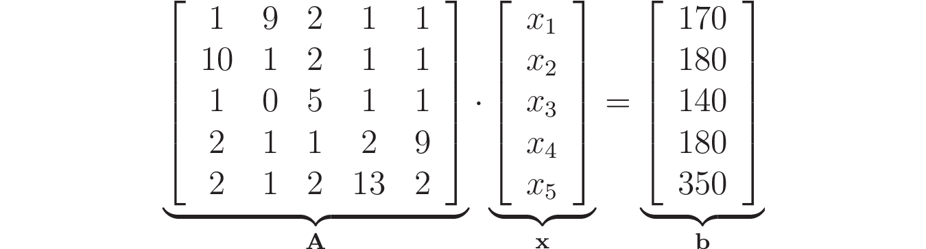
Scipy.linalg.solve () can now be used to solve the system:
>>>

In [1]: import numpy as np

   ...: from scipy.linalg import solve

In [2]: A = np.array(

   ...:    [

   ...:        [1, 9, 2, 1, 1],

   ...:        [10, 1, 2, 1, 1],

   ...:        [1, 0, 5, 1, 1],

   ...:        [2, 1, 1, 2, 9],

   ...:        [2, 1, 2, 13, 2],

   ...:    ]

   ...: )

In [3]: b = np.array([170, 180, 140, 180, 350]).reshape((5, 1))

In [4]: x = solve(A, b)

   ...: x

Out[4]:

array([[10.],

       [10.],

       [20.],

       [20.],

       [10.]])
We got the result. Let's decipher it. A balanced diet should include:
- 10 units of product 1;
- 10 units of product 2;
- 20 units of product 3;
- 20 units of product 4;
- 10 units of product 5.
Eat right! Use scipy.linalg and be healthy!
Cloud VPS servers with fast NVM drives and daily payment. Upload your ISO.