Mushrooms (Machine Learning)

Hello everyone! Consider the data on mushrooms, predict their edibility, build a correlation, and much more.

We will use data on mushrooms from Kaggle (original dataframe) from  https://www.kaggle.com/uciml/mushroom-classification , 2 additional dataframes will be attached to the article.

All operations are done at  https://colab.research.google.com/notebooks/intro.ipynb

#  e    
import pandas as pd

#     ,     confusion_matrix:
from sklearn.ensemble import RandomForestClassifier
from sklearn.model_selection import GridSearchCV
from sklearn.metrics import confusion_matrix

#    :
import matplotlib.pyplot as plt
import seaborn as sns

#   
mushrooms = pd.read_csv('/content/mushrooms.csv')

#  
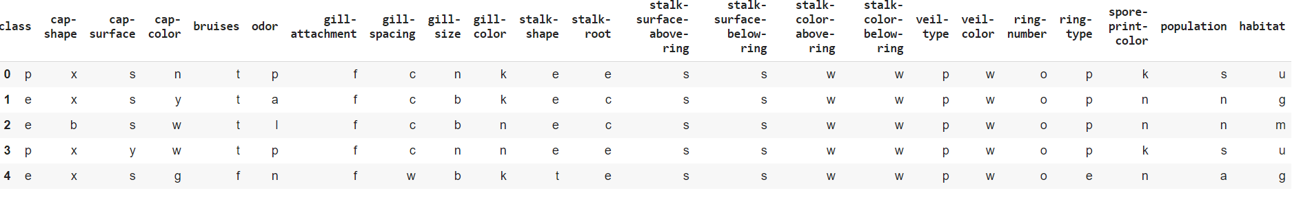
mushrooms.head()
#           :
      
      

        
        
        
      

    
        
        
        
      
      

        
        
        
      

    
    

#  
mushrooms.info()
      
      

        
        
        
      

    
        
        
        
      
      

        
        
        
      

    
    

#     
mushrooms.shape

#    LabelEncoder          (  heatmap)
#     ,           
from sklearn.preprocessing import LabelEncoder
le=LabelEncoder()
for i in mushrooms.columns:
    mushrooms[i]=le.fit_transform(mushrooms[i])

#     
mushrooms.head()
      
      

        
        
        
      

    
        
        
        
      
      

        
        
        
      

    
    

#       heatmap
fig = plt.figure(figsize=(18, 14))
sns.heatmap(mushrooms.corr(), annot = True, vmin=-1, vmax=1, center= 0, cmap= 'coolwarm', linewidths=3, linecolor='black')
fig.tight_layout()
plt.show()
      
      

        
        
        
      

    
        
        
        
      
      

        
        
        
      

    
    

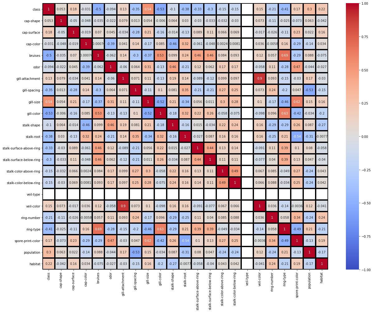
: (veil-color,gill-spacing) = +0.9 (ring-type,bruises) = +0.69 (ring-type,gill-color) = +0.63 (spore-print-color,gill-size) = +0.62 (stalk-root,spore-print-color) = -0.54 (population,gill-spacing) = -0.53 (gill-color,class) = -0.53 , . , , .

#  ,   .
X = mushrooms.drop(['class'], axis=1)
#  ,   .
y = mushrooms['class']

#   RandomForestClassifier.
rf = RandomForestClassifier(random_state=0)

#   ,            
#{'n_estimators': range(10, 51, 10), 'max_depth': range(1, 13, 2),
#             'min_samples_leaf': range(1,8), 'min_samples_split': range(2,10,2)}
parameters = {'n_estimators': [10], 'max_depth': [7],
              'min_samples_leaf': [1], 'min_samples_split': [2]}

#  Random forest  GridSearchCV.
GridSearchCV_clf = GridSearchCV(rf, parameters, cv=3, n_jobs=-1)
GridSearchCV_clf.fit(X, y)

#   ,          
best_clf = GridSearchCV_clf.best_params_

#   .
best_clf
      
      

        
        
        
      

    
        
        
        
      
      

        
        
        
      

    
    

#  confusion matrix ( )  ,          .
y_true = pd.read_csv ('/content/testing_y_mush.csv')
sns.heatmap(confusion_matrix(y_true, predictions), annot=True, cmap="Blues")
plt.show()
      
      

        
        
        
      

    
        
        
        
      
      

        
        
        
      

    
    

This matrix of errors shows that we have no errors of the first type, but there are errors of the second type in the value 3, which for our model is a very low indicator tending to 0.

Next, we will perform operations to determine the model of the best accuracy for our df

#     
from sklearn.metrics import accuracy_score
mr = accuracy_score(y_true, predictions)


#     
from sklearn.model_selection import train_test_split
x_train, x_test, y_train, y_test = train_test_split(X, y, test_size = 0.2, random_state = 0)

# 
# 
from sklearn.linear_model import LogisticRegression
lr = LogisticRegression(max_iter = 10000)
lr.fit(x_train,y_train)

#  
from sklearn.metrics import confusion_matrix,classification_report
y_pred = lr.predict(x_test)
cm = confusion_matrix(y_test,y_pred)


#  
log_reg = accuracy_score(y_test,y_pred)


#K  
# 
from sklearn.neighbors import KNeighborsClassifier
knn = KNeighborsClassifier(n_neighbors = 5, metric = 'minkowski',p = 2)
knn.fit(x_train,y_train)

#  
from sklearn.metrics import confusion_matrix,classification_report
y_pred = knn.predict(x_test)
cm = confusion_matrix(y_test,y_pred)


#  
from sklearn.metrics import accuracy_score
knn_1 = accuracy_score(y_test,y_pred)


# 
# 
from sklearn.tree import DecisionTreeClassifier
dt = DecisionTreeClassifier(criterion = 'entropy')
dt.fit(x_train,y_train)

#  
from sklearn.metrics import confusion_matrix,classification_report
y_pred = dt.predict(x_test)
cm = confusion_matrix(y_test,y_pred)

#  
from sklearn.metrics import accuracy_score
dt_1 = accuracy_score(y_test,y_pred)


#  
# 
from sklearn.naive_bayes import GaussianNB
nb = GaussianNB()
nb.fit(x_train,y_train)

#  
from sklearn.metrics import confusion_matrix,classification_report
y_pred = nb.predict(x_test)
cm = confusion_matrix(y_test,y_pred)


#  
from sklearn.metrics import accuracy_score
nb_1 = accuracy_score(y_test,y_pred)


#  
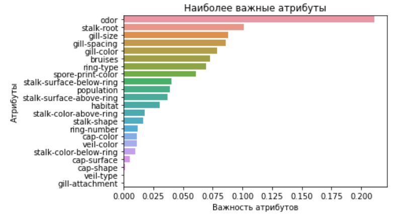
plt.figure(figsize= (16,12))
ac = [log_reg,knn_1,nb_1,dt_1,mr]
name = [' ','  ','  ',' ', ' ']
sns.barplot(x = ac,y = name,palette='colorblind')
plt.title("  ", fontsize=20, fontweight="bold")
      
      

        
        
        
      

    
        
        
        
      
      

        
        
        
      

    
    

We can conclude that the most accurate model for our predictions is a decision tree.