Good day, dear Habradams and Habragospoda. In this article, we will close the hatches of our bathyscaphe as tightly as possible, add speed to our Python engine and plunge into the abyss of statistics, to a depth into which sunlight practically does not penetrate. At this depth, we will encounter a lot of all kinds of statistical tests that float past us in the form of bizarre formulas. At first it will seem to us that they are all arranged differently, but we will try to get to the bottom of the main driving force of all these strange creatures.
What should I warn you about before diving to this depth? First, I assume that you have already read the book "Statistics for All" by Sarah Boslaf, and also rummaged in the official documentation of the stats module of the SciPy library. Forgive me for my next guess, but it seems to me that you were most likely a little dumbfounded by the sheer number of tests that are out there, and were dumbfounded even more when you realized that this is really just the tip of the iceberg. Well, if you have not yet encountered all the delights of this wonderful "puberty", then I recommend getting the book by Alexander Ivanovich Kobzar "Applied Mathematical Statistics. For Engineers and Scientists." Well, if you are "in the subject", then still look under the cat,why? Because the presentation and interpretation of facts is sometimes more important and interesting than the facts themselves.
, :
import numpy as np
import pandas as pd
from scipy import stats
import matplotlib.pyplot as plt
import seaborn as sns
from pylab import rcParams
sns.set()
rcParams['figure.figsize'] = 10, 6
%config InlineBackend.figure_format = 'svg'
np.random.seed(42)
, , . , , - , , . [0; 10] 0 - "", 10 - " ". , :
![x_ {1} = [7.68, \; \; 5.40, \; \; 3.99, \; \; 3.27, \; \; 2.70, \; \; 5.85, \; \; 6.53, \; \; 5.00, \; \; 4.60, \; \; 6.18]](https://habrastorage.org/getpro/habr/upload_files/148/fc2/b25/148fc2b253952e2994d7a369321c13dd.svg)
- , - , - . :
![x_ {2} = [1.33, \; \; 1.66, \; \; 2.76, \; \; 4.56, \; \; 4.75, \; \; 0.70, \; \; 3.13, \; \; 1.96, \; \; 4.60, \; \; 3.69]](https://habrastorage.org/getpro/habr/upload_files/2ef/3a1/e2c/2ef3a1e2c921ee1c0773552e277b2276.svg)
, , , . , . , . , .. . " Pthon - " -.
, , . " , , ", - , , . , : , , .. .. , :
" " ;
" " ;
" " .
, . , , . :
x1 = np.array([7.68,5.40,3.99,3.27,2.70,5.85,6.53,5.00,4.60,6.18])
x2 = np.array([1.33,1.66,2.76,4.56,4.75,0.70,3.13,1.96,4.60,3.69])
fig, ax = plt.subplots()
sns.ecdfplot(x=x1, ax=ax, label=' ')
sns.ecdfplot(x=x2, ax=ax, label='')
ax.legend();
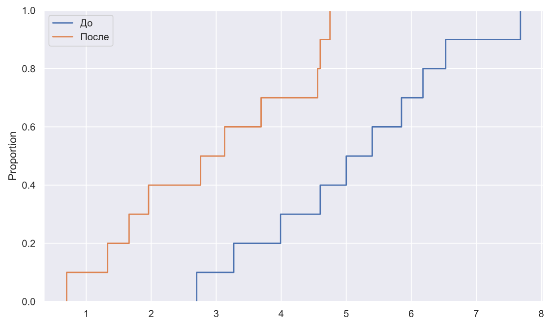
, , ( ), , :
plt.bar(np.arange(10), (x2-x1));
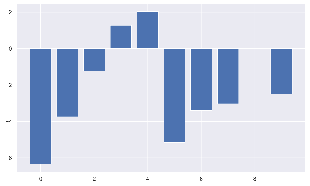
, - . , , , . , :
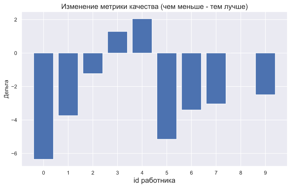
plt.bar(np.arange(10), (x2-x1))
plt.xticks(np.arange(10));
plt.title(' ( - )',
fontsize=15)
plt.xlabel('id ', fontsize=15)
plt.ylabel('');
:
plt.bar(np.arange(10) - 0.2, x1, width=0.4, label='')
plt.bar(np.arange(10) + 0.2, x2, width=0.4, label='')
plt.xticks(np.arange(10))
plt.legend()
plt.title(' ( - )',
fontsize=15)
plt.xlabel('id ', fontsize=15)
plt.ylabel('');
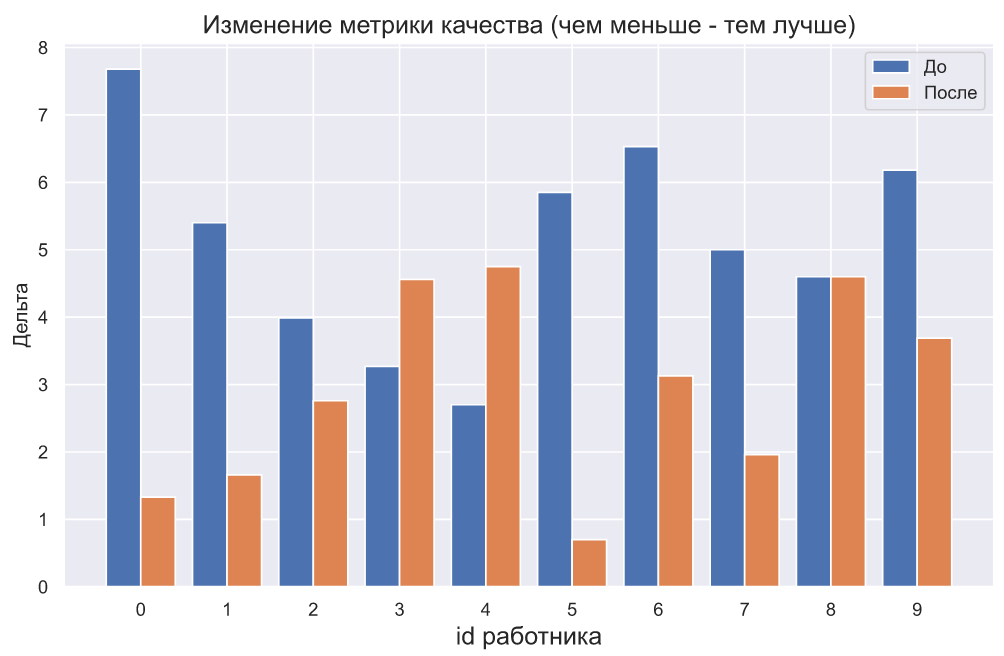
, - , , , . , . , , , , . - .
, - t- :
stats.ttest_rel(x2, x1)
Ttest_relResult(statistic=-2.5653968678354184, pvalue=0.03041662395965993)
 c p-value 0.03 , . , . - . ?
:
print(f'mean(x1) = {x1.mean():.3}')
print(f'mean(x2) = {x2.mean():.3}')
print('-'*15)
print(f'std(x1) = {x1.std(ddof=1):.3}')
print(f'std(x2) = {x2.std(ddof=1):.3}')
mean(x1) = 5.12
mean(x2) = 2.91
---------------
std(x1) = 1.53
std(x2) = 1.47
t- , , (, ), . ? , ? ? , , .. , . , ?
( ) - -. , () , . , - . - , . , , - - . - , .
, t- , , . , . , . , ?
, . 5000 
 10 , :
samples = stats.norm.rvs(loc=(5, 3), scale=1.5, size=(5000, 10, 2))
deviations = samples.var(axis=1, ddof=1)
deviations_df = pd.DataFrame(deviations, columns=['s1', 's2'])
sns.histplot(data=deviations_df, element="poly", color='r', fill=False);
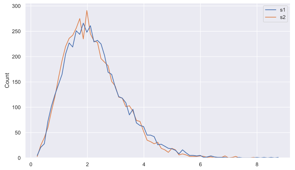
, , "" - . :
sns.histplot(data=pd.DataFrame(np.std(stats.norm.rvs(loc=(5, 3), scale=1.5, size=(5000,10,2)), axis=1, ddof=1), columns=['s1', 's2']), element="poly", color='r', fill=False);
"" - . - , , :
- ;
;
, .
, - "", "". " ", .. . , , , . , .
, . , , , . : "" . , ", " - , - . , fit():
df1, loc1, scale1 = stats.chi2.fit(deviations_df['s1'], fdf=10)
print(f'df1 = {df1}, loc1 = {loc1:<8.4}, scale1 = {scale1:.3}')
df2, loc2, scale2 = stats.chi2.fit(deviations_df['s2'], fdf=10)
print(f'df2 = {df2}, loc2 = {loc2:<8.4}, scale1 = {scale2:.3}')
df1 = 10, loc1 = -0.1027 , scale1 = 0.238
df2 = 10, loc2 = -0.08352, scale1 = 0.231
fig, ax = plt.subplots()
# ,
# 0.5 1:
sns.histplot(data=deviations_df['s1'], color='r', element='poly',
fill=False, stat='density', label='s1', ax=ax)
sns.histplot(data=deviations_df['s2'], color='b', element='poly',
fill=False, stat='density', label='s2', ax=ax)
chi2_rv1 = stats.chi2(df1, loc1, scale1)
chi2_rv2 = stats.chi2(df2, loc2, scale2)
x = np.linspace(0, 8, 300)
sns.lineplot(x=x, y=chi2_rv1.pdf(x), color='r', label='pdf(s1)', ax=ax)
sns.lineplot(x=x, y=chi2_rv2.pdf(x), color='b', label='pdf(s2)', ax=ax)
ax.set_xticks(np.arange(10))
ax.set_xlabel('s');
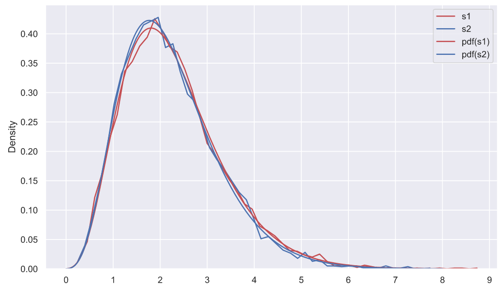
- . , , , , , , ( ). . , (""), ("") ("") (""), , , . , , , "" , , .
? , , 
 . , . ? , 2,
  ?
?
fig, ax = plt.subplots()
var = 2**2
x = np.linspace(0, 10, 300)
sns.lineplot(x=x, y=chi2_rv1.pdf(x), label='pdf(s1)', ax=ax)
ax.vlines(var, 0, chi2_rv1.pdf(var), color='r', lw=2)
ax.fill_between(x[x>var], chi2_rv1.pdf(x[x>var]),
np.zeros(len(x[x>var])), alpha=0.3, color='b')
ax.hlines(0, x.min(), x.max(), lw=1, color='k')
p = chi2_rv1.sf(var)
ax.set_title(f'$P(s_{1} \geqslant {var}) = $' + '{:.3}'.format(p))
ax.set_xlabel('s');
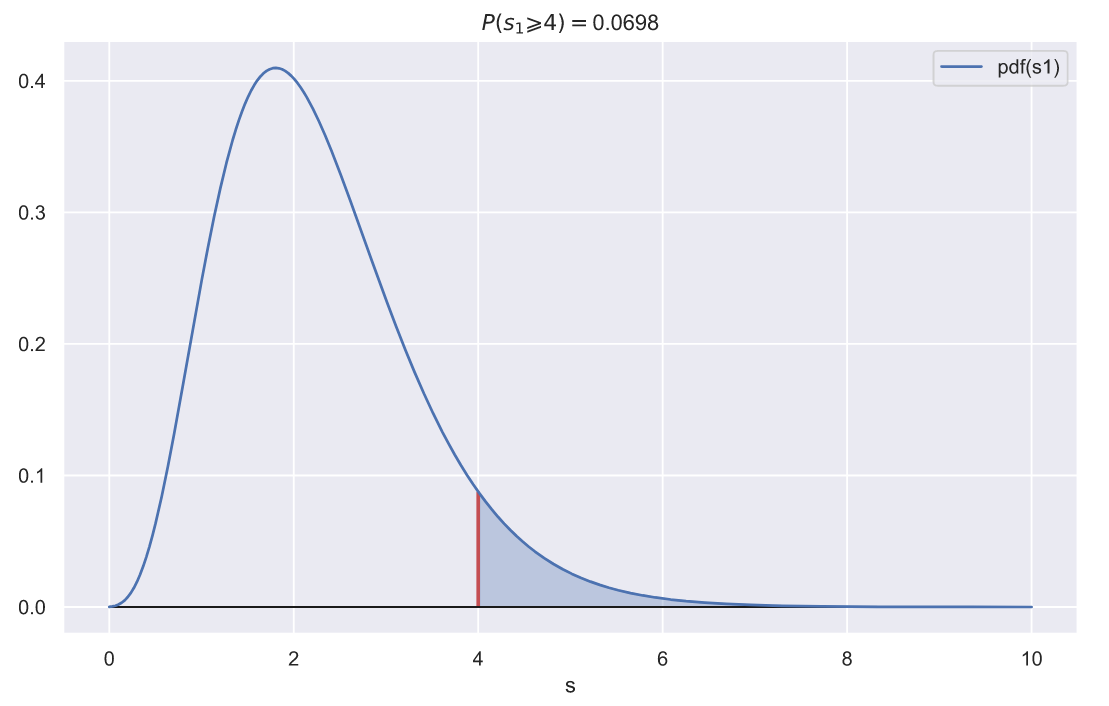
p-value , , , 10 
 . ,
. ,  1.5. ,
  , - , .
, - , , 0.1:
fig, ax = plt.subplots()
x = np.linspace(0, 10, 300)
sns.lineplot(x=x, y=chi2_rv1.pdf(x), label='pdf(s1)', ax=ax)
# :
ci_left, ci_right = chi2_rv1.interval(0.9)
ax.vlines([ci_left, ci_right], 0, 0.5, color='r', lw=2)
x_le_ci_l, x_ge_ci_r = x[x<ci_left], x[x>ci_right]
ax.fill_between(x_le_ci_l, chi2_rv1.pdf(x_le_ci_l),
np.zeros(len(x_le_ci_l)), alpha=0.3, color='b')
ax.fill_between(x_ge_ci_r, chi2_rv1.pdf(x_ge_ci_r),
np.zeros(len(x_ge_ci_r)), alpha=0.3, color='b')
ax.set_title(f'P({ci_left:.3} $\geqslant s_{1} \geqslant$ {ci_right:.3}) = 0.1')
ax.hlines(0, x.min(), x.max(), lw=1, color='k')
ax.set_xlabel('s');
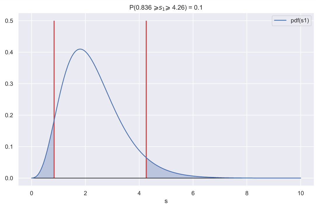
,  , - , , .
? , - . , :

 :
:
rel_dev = deviations_df['s1'] / deviations_df['s2']
sns.histplot(x=rel_dev, stat='density');
, fit():
dfn, dfd, loc, scale = stats.f.fit(rel_dev, fdfn=10, fdfd=10)
print(f'dfn = {dfn}, dfd = {dfd}, loc2 = {loc2:<8.4}, scale1 = {scale2:.3}')
dfn = 10, dfd = 10, loc2 = -0.08352, scale1 = 0.231
fig, ax = plt.subplots()
rel_dev = deviations_df['s1'] / deviations_df['s2']
sns.histplot(x=rel_dev, stat='density', alpha=0.4)
f_rv = stats.f(dfn, dfd, loc, scale)
x = np.linspace(0, 12, 300)
ax.plot(x, f_rv.pdf(x), color='r')
ax.set_xlim(0, 8);

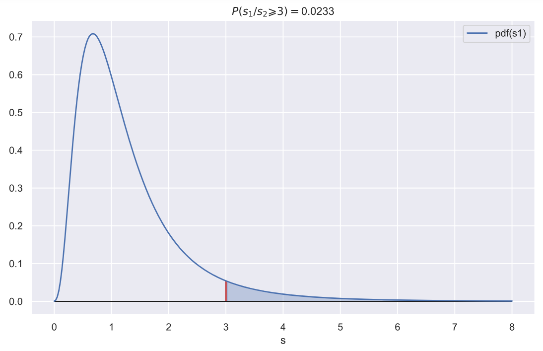
. , 3, 1, :
fig, ax = plt.subplots()
rel_var = 3
x = np.linspace(0, 8, 300)
sns.lineplot(x=x, y=f_rv.pdf(x), label='pdf(s1)', ax=ax)
ax.vlines(rel_var, 0, f_rv.pdf(rel_var), color='r', lw=2)
ax.fill_between(x[x>rel_var], f_rv.pdf(x[x>rel_var]),
np.zeros(len(x[x>rel_var])), alpha=0.3, color='b')
ax.hlines(0, x.min(), x.max(), lw=1, color='k')
p = f_rv.sf(var)
ax.set_title(f'$P(s_{1}/s_{2} \geqslant {rel_var}) = $' + '{:.3}'.format(p))
ax.set_xlabel('s');
, 10 
 , , 3, 0.023. , .
:
np.var(x1, ddof=1) / np.var(x2, ddof=1)
1.083553459313125
. , , . , ? ANOVA? , , , , . f_oneway() ( pvalue, , ):
stats.f_oneway(x1, x2)
F_onewayResult(statistic=10.786061383971454, pvalue=0.0041224402038065235)
? - ?
, f_oneway(), :


m1, m2, m = *np.mean((x1, x2), axis=1), np.mean((x1, x2))
ms_bg = (10*(m1 - m)**2 + 10*(m2 - m)**2)/(2 - 1)
ms_wg = (np.sum((x1 - m1)**2) + np.sum((x2 - m2)**2))/(20 - 2)
s = ms_bg/ms_wg
p = stats.f.sf(s, dfn=1, dfd=18)
print(f'statistic = {s:.5}, p-value = {p:.5}')
statistic = 10.786, p-value = 0.0041224
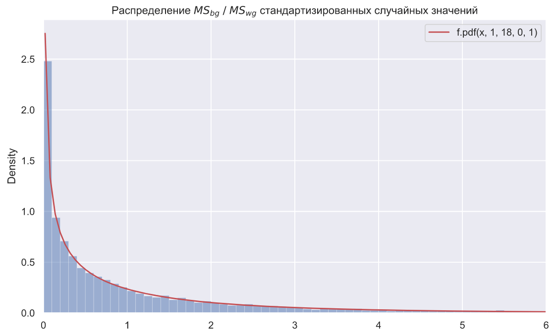
 (mean square between group) , . , ,
  .
.  (mean square within group) , , . , , , . , - , , . , ,
 :
:

:
N = 10000
samples_1 = stats.norm.rvs(loc=0, scale=1, size=(N, 10))
samples_2 = stats.norm.rvs(loc=0, scale=1, size=(N, 10))
m1 = samples_1.mean(axis=1)
m2 = samples_2.mean(axis=1)
m = np.hstack((samples_1, samples_2)).mean(axis=1)
ms_bg = 10*((m1 - m)**2 + (m2 - m)**2)
ss_1 = np.sum((samples_1 - m1.reshape(N, 1))**2, axis=1)
ss_2 = np.sum((samples_2 - m2.reshape(N, 1))**2, axis=1)
ms_wg = (ss_1 + ss_2)/18
statistics = ms_bg/ms_wg
f, ax = plt.subplots()
x = np.linspace(0.02, 30, 500)
plt.plot(x, stats.f.pdf(x, dfn=1, dfd=18), color='r', label=f'f.pdf(x, 1, 18, 0, 1)')
plt.legend()
sns.histplot(x=statistics, binwidth=0.1, stat='density', alpha=0.5)
ax.set_xlim(0, 6)
ax.set_title(r' $MS_{bg} \; / \;MS_{wg}$ ');
N = 10000
mu_1 = stats.uniform.rvs(loc=0, scale=5, size=(N, 1))
samples_1 = stats.norm.rvs(loc=mu_1, scale=2, size=(N, 10))
mu_2 = stats.uniform.rvs(loc=0, scale=5, size=(N, 1))
samples_2 = stats.norm.rvs(loc=mu_2, scale=2, size=(N, 10))
m1 = samples_1.mean(axis=1)
m2 = samples_2.mean(axis=1)
m = np.hstack((samples_1, samples_2)).mean(axis=1)
ms_bg = 10*((m1 - m)**2 + (m2 - m)**2)
ss_1 = np.sum((samples_1 - m1.reshape(N, 1))**2, axis=1)
ss_2 = np.sum((samples_2 - m2.reshape(N, 1))**2, axis=1)
ms_wg = (ss_1 + ss_2)/18
statistics = ms_bg/ms_wg
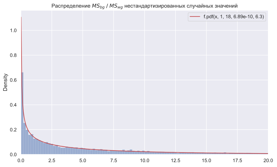
loc, scale = stats.f.fit(statistics, fdfn=1, fdfd=18)[-2:]
f, ax = plt.subplots()
x = np.linspace(0.02, 30, 500)
plt.plot(x, stats.f.pdf(x, dfn=1, dfd=18, loc=loc, scale=scale), color='r', label=f'f.pdf(x, 1, 18, {loc:.3}, {scale:.3})')
plt.legend()
sns.histplot(x=statistics, binwidth=0.2, stat='density', alpha=0.5)
ax.set_xlim(0, 20)
ax.set_title(r' $MS_{bg} \; / \;MS_{wg}$ ');
, SciPy levene(). () , ANOVA, :
stats.levene(x1, x2)
LeveneResult(statistic=0.0047521397921121405, pvalue=0.9458007897725039)
""
, , . , , , , , . , , . : 10000 5 , , , :
N, k = 10000, 5
func = [stats.uniform, stats.norm, stats.laplace]
color = list('gyb')
labels = ['s_uniform', 's_norm', 's_laplace']
for i in range(3):
ss = np.square(func[i].rvs(size=(N, k))).sum(axis=1)
sns.histplot(x=ss, stat='density', label=labels[i] + '.pdf(x)',
element='step', color=color[i], lw=2, fill=False)
x = np.linspace(0, 25, 300)
plt.plot(x, stats.chi2.pdf(x, df=5), color='r', label='chi2.pdf(x, df=5)')
plt.legend()
plt.xlim(0, 20);
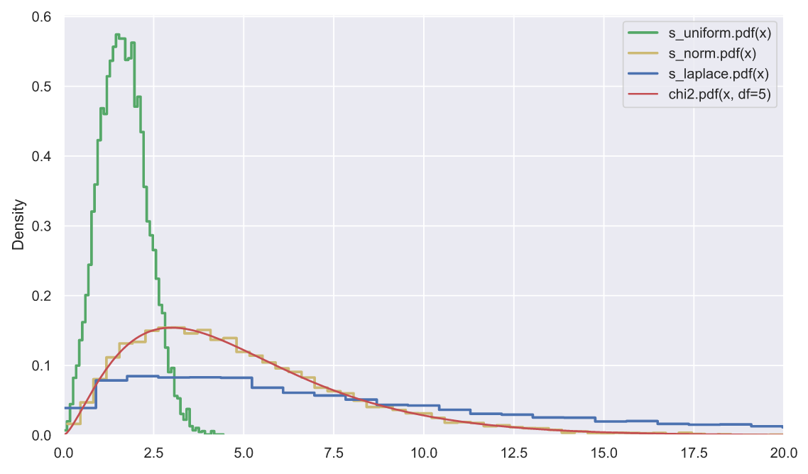
, - , , , "" . , , , - (- - ).
- ANOVA, , "" ? , :
array([0.40572556, 0.67443266, 0.38765587, 0.96540199, 0.57933085])
, - . ? 50 5 , , , :
s = np.sort(stats.norm.rvs(size=(50000, 5)), axis=1).T
for i in range(5):
sns.histplot(x=s[i], stat='density',
label='i = ' + str(i),
element='poly', lw=2, fill=False)
plt.xticks(np.arange(-5, 6))
plt.legend();
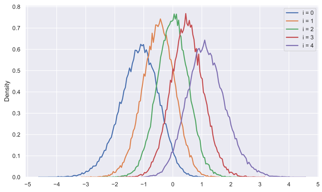
, ? , , , . , :
" " ;
;
( );
- , ( );
.
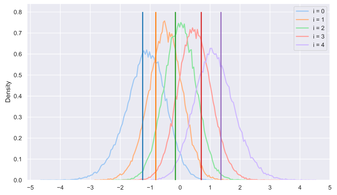
, , , , "" . ?!! , , - :
s = np.sort(stats.norm.rvs(size=(50000, 5)), axis=1).T
sample = np.sort(stats.norm.rvs(size=5))
colors = sns.color_palette('tab10', 5)
for i in range(5):
sns.histplot(x=s[i], stat='density',
label='i = ' + str(i),
element='poly', lw=2, fill=False,
color=sns.color_palette('pastel', 5)[i])
plt.vlines(sample[i], 0, 0.8, lw=2, zorder=10,
color=sns.color_palette('tab10', 5)[i])
plt.xticks(np.arange(-5, 6))
plt.legend();
- :
s = np.sort(stats.norm.rvs(size=(50000, 5)), axis=1).T
sample = np.sort(stats.uniform.rvs(loc=-2, scale=4, size=5))
colors = sns.color_palette('tab10', 5)
for i in range(5):
sns.histplot(x=s[i], stat='density',
label='i = ' + str(i),
element='poly', lw=2, fill=False,
color=sns.color_palette('pastel', 5)[i])
plt.vlines(sample[i], 0, 0.8, lw=2, zorder=10,
color=sns.color_palette('tab10', 5)[i])
plt.xticks(np.arange(-5, 6))
plt.legend();
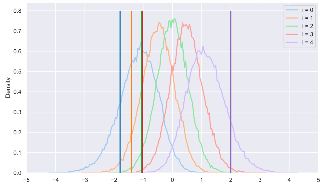
, - . , , - . : , . , . , . :
stats.ks_1samp(x1, stats.norm.cdf, args=(5, 1.5))
KstestResult(statistic=0.11452966409855592, pvalue=0.9971279018404035)
, p-value, , "" . , , . , , :
x1.sort()
n = len(x1)
ecdf_ge = np.r_[1:n+1]/n
ecdf_le = np.r_[0:n]/n
cdf_teor = stats.norm.cdf(x1, loc=5, scale=1.5)
plt.plot(x1, ecdf_ge, color='b', drawstyle='steps-post', label='ecdf_ge')
plt.plot(x1, cdf_teor, color='r', drawstyle='steps-post', label='cdf_teor')
plt.plot(x1, ecdf_le, color='g', drawstyle='steps-post', label='ecdf_le')
plt.legend();
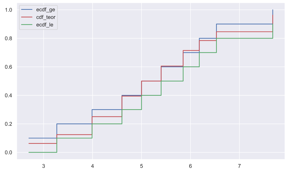
, .. :
d_plus = ecdf_ge - cdf_teor d_minus = cdf_teor - ecdf_le statistic = np.max([d_plus, d_minus]) statistic
0.11452966409855592
( n=5):
x = np.linspace(0, 1, 3000)
plt.plot(x, stats.kstwo.pdf(x, n));
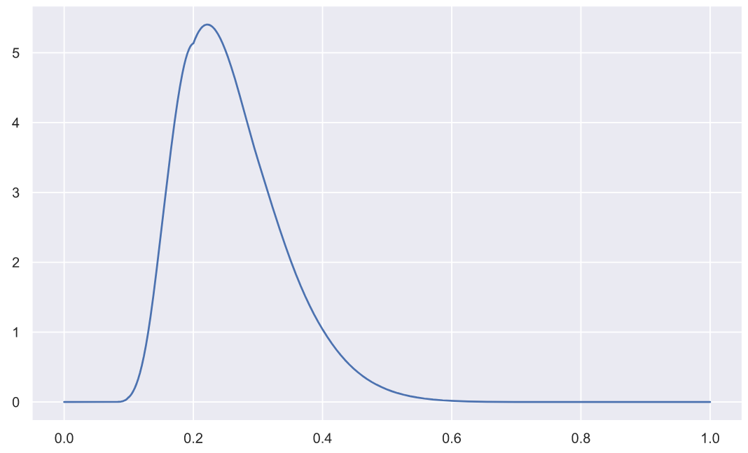
p-value:
pvalue = stats.kstwo.sf(statistic, n) pvalue
0.9971279018404035
, . , , ecdf_le ( ). , ecdf_le . , "" , seaborn, , .
, , -, , : " ?" , : " , ?" , . , - , , ? , . , - ? , .
Scientific and technical articles are not easy reading, but writing them is even more tedious. I would like to convey some complex ideas in a simple and relaxed way. I would like to hope that I can do it at least a little.
Nevertheless, be that as it may, we will continue to dive! In Eminem's song "My name is" I have a favorite line "I just drank a fifth of vodka - dare me to drive? (Go ahead)", which fits very well for the whole dive.
As usual, I press F5 and look forward to your comments!