1. Introduction
When performing engineering and geological surveys, a task may arise related to comparing data from field and laboratory studies on the same soils in order to confirm the correct transportation of samples from the survey object to the laboratory (the samples were not deformed and / or destroyed during transportation).
With this formulation of the problem, you can apply the A / B testing technique with the following parameters:
The measured metric will be the average value of the density of the soil skeleton (p d , g / cm 3 ), which characterizes the addition of samples. This value has a normal distribution law;
The criterion for testing the hypothesis will be the t-test (Student's test): for two independent samples , if the compared field (before transportation) and laboratory (after transportation) data were carried out on different soil samples; for two dependent samples , if the studies were performed on the same samples.
Within the framework of this topic, we will generate two random samples, which we will compare, formulate statistical hypotheses, test them and draw conclusions.
2. Generation of samples
2.1 Estimation of sample size
As part of the design of the experiment, before generating the density samples, let us estimate their required volume for a given effect size (ES - effect size) , power and allowable type I error (α) (definitions of these terms are given below). We will make the calculation using the statsmodels package .
Effect size (standardized) is the value that characterizes the difference we want to detect, equal to the ratio of the difference in the mean values across the samples to the weighted standard deviation. In our case:


The weighted standard deviation S pooled for samples of the same size can be calculated using the formula:

(Cohen, 1988) ES = 0.2 - ; 0.5 - ; 0.8 - .
– II ( 80%).
I II :
H0 |
H1 |
|
|---|---|---|
H0 |
H0 |
II (β) |
H0 |
I (α) |
H0 (power = 1-β) |
:
α = 0.05 ( )
ES = 0.5 ( ).
Power = 0.8 ( ).
:
#
import numpy as np
from statsmodels.stats.power import TTestIndPower

from matplotlib.pyplot import figure
import matplotlib.pyplot as plt

import scipy
from statsmodels.stats.weightstats import *
#
effect = 0.5
alpha = 0.05
power = 0.8

analysis = TTestIndPower()

#
size = analysis.solve_power(effect, power=power, alpha=alpha)

print(f' , .: {int(size)}')
, .: 63
, 63 . 65 .
.
plt.figure(figsize=(10, 7), dpi=80)

results = dict((i/10, analysis.solve_power(i/10, power=power, alpha=alpha))
               for i in range(2, 16, 1))

plt.plot(list(results.keys()), list(results.values()), 'bo-')

plt.grid()
plt.title('     \n   ')
plt.ylabel('  n, .')
plt.xlabel('  ES, ..')

for x,y in zip(list(results.keys()),list(results.values())):

    label = "{:.0f}".format(y)

    plt.annotate(label,
                 (x,y),
                 textcoords="offset points",
                 xytext=(0,10),
                 ha='center')

plt.show()
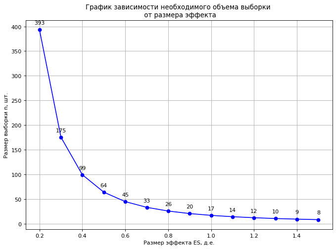
, ES. : 0,03 /3 0,1 /c3 (ES = 0,03 /3 / 0,1 /3 = 0,3 ..), 175 (power=0.80, α=0.05).
2.2
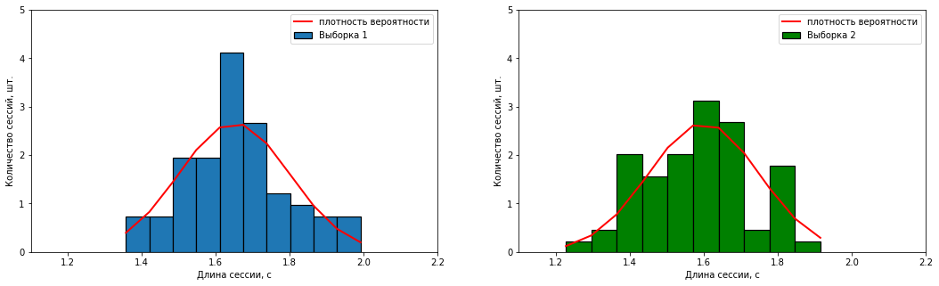
, numpy.
( ) . (X̄) (S):
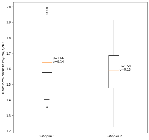
– X̄1= 1,65 /3, S1 = 0.15 /3;
– X̄2 = 1,60 /3, S2 = 0.15 /3.
loc_1 = 1.65
sigma_1 = 0.15

loc_2 = 1.60
sigma_2 = 0.15

sample_size = 65
#
sample_1 = np.random.normal(loc=loc_1, scale=sigma_1, size=sample_size)
sample_2 = np.random.normal(loc=loc_2, scale=sigma_2, size=sample_size)
" " .
fig, axes = plt.subplots(ncols=2, figsize=(18, 5))

max_y = np.max(np.hstack([sample_1,sample_2]))
#   1
count_1, bins_1, ignored_1 = axes[0].hist(sample_1, 10, density=True,
                                          label=" 1", edgecolor='black',
                                          linewidth=1.2)
axes[0].plot(bins_1, 1/(sigma_1 * np.sqrt(2 * np.pi)) *
               np.exp( - (bins_1 - loc_1)2 / (2 * sigma_12)),
         linewidth=2, color='r', label=' ')
axes[0].legend()
axes[0].set_xlabel(u' , ')
axes[0].set_ylabel(u' , .')
axes[0].set_ylim([0, 5])
axes[0].set_xlim([1.1, 2.2])

#   2
count_2, bins_2, ignored_2 = axes[1].hist(sample_2, 10, density=True,
                                          label=" 2", edgecolor='black',
                                          linewidth=1.2, color="green")
axes[1].plot(bins_2, 1/(sigma_2 * np.sqrt(2 * np.pi)) *
               np.exp( - (bins_2 - loc_2)2 / (2 * sigma_22)),
         linewidth=2, color='r', label=' ')
axes[1].legend()
axes[1].set_xlabel(u' , ')
axes[1].set_ylabel(u' , .')
axes[1].set_ylim([0, 5])
axes[1].set_xlim([1.1, 2.2])
plt.show()
#
fig, ax = plt.subplots(figsize=(8, 8))
axis = ax.boxplot([sample_1, sample_2], labels=[' 1', ' 2'])

data = np.array([sample_1, sample_2])
means = np.mean(data, axis = 1)
stds = np.std(data, axis = 1)

for i, line in enumerate(axis['medians']):
    x, y = line.get_xydata()[1]
    text = ' μ={:.2f}\n σ={:.2f}'.format(means[i], stds[i])
    ax.annotate(text, xy=(x, y))

plt.ylabel('  , /3')
plt.show()
3.
. :
1. , t- ;
2. , t- .
.
1.
.
H0: μ1 = μ2.
H1: μ1≠μ2.
:

: T(X1n1,X2n2)≈~St(ν), ν

ttest_ind stats.
t_st, p_val = scipy.stats.ttest_ind(sample_1, sample_2, equal_var = False)
print(f't-  {round(t_st, 2)}')
print(f' t-   \
  (p-value)  {round(p_val, 3)}')
t- 2.92
t- (p-value) 0.004
№ 1
H0 , , 0,05 ( p-value 0.004) .
.
c_m = CompareMeans(DescrStatsW(sample_1), DescrStatsW(sample_2))
print("95%%  : \
[%.4f, %.4f]" % c_m.tconfint_diff(usevar='unequal'))
95% : [0.0235, 0.1228]
95% , , 5%.
2.
, ( ) ( ) . , .
H0: μ1 = μ2.
H1: μ1≠μ2.
:


: T(X1n, X2n) ~ St(n-1)
ttest_rel stats.
t_st, p_val = stats.ttest_rel(sample_1, sample_2)
print(f't-  {round(t_st, 2)}')
print(f' t-   \
  (p-value)  {round(p_val, 3)}')
t- 2.79
t- (p-value) 0.007
№ 2
H0 , , 0,05 ( p-value 0.007).
For clarity, let's also estimate the interval between the means for these samples.
print("95%% confidence interval: [%.4f, %.4f]"
      % DescrStatsW(sample_1 - sample_2).tconfint_mean())
95% confidence interval: [0.0208, 0.1255]
Since zero does not fall within the considered 95% confidence interval, we can conclude that the mean values of the considered samples differ.
5. Outcome
In this article, we examined the possibility of using the Python language in solving a practical problem in engineering geology, with an accompanying study of the issue of the required sample size for testing hypotheses.