Good day, habraledi and habragentelmen! In this article, we'll continue our dive into statistics with Python. If anyone missed the start of the dive, here's a link to the first part . Well, if not, I still recommend keeping Sarah Boslaf's open book, Statistics for All, close at hand. I also recommend running notepad to experiment with code and graphs.
As Andrew Lang said, “ Statistics are to a politician like a street lamp to a drunken bummer: a prop rather than a lighting. ” The same can be said for this article for newbies. It is unlikely that you will learn a lot of new knowledge here, but I hope this article will help you understand how to use Python to facilitate self-study of statistics.
Why invent new allocations?
Imagine ... so, before we imagine anything, let's do all the necessary imports again:
import numpy as np
from scipy import stats
import matplotlib.pyplot as plt
import seaborn as sns
from pylab import rcParams
sns.set()
rcParams['figure.figsize'] = 10, 6
%config InlineBackend.figure_format = 'svg'
np.random.seed(42)
, , . , , - , . 1000 100- , . :
gen_pop = np.trunc(stats.norm.rvs(loc=80, scale=5, size=1000))
gen_pop[gen_pop>100]=100
print(f'mean = {gen_pop.mean():.3}')
print(f'std = {gen_pop.std():.3}')
mean = 79.5
std = 4.95
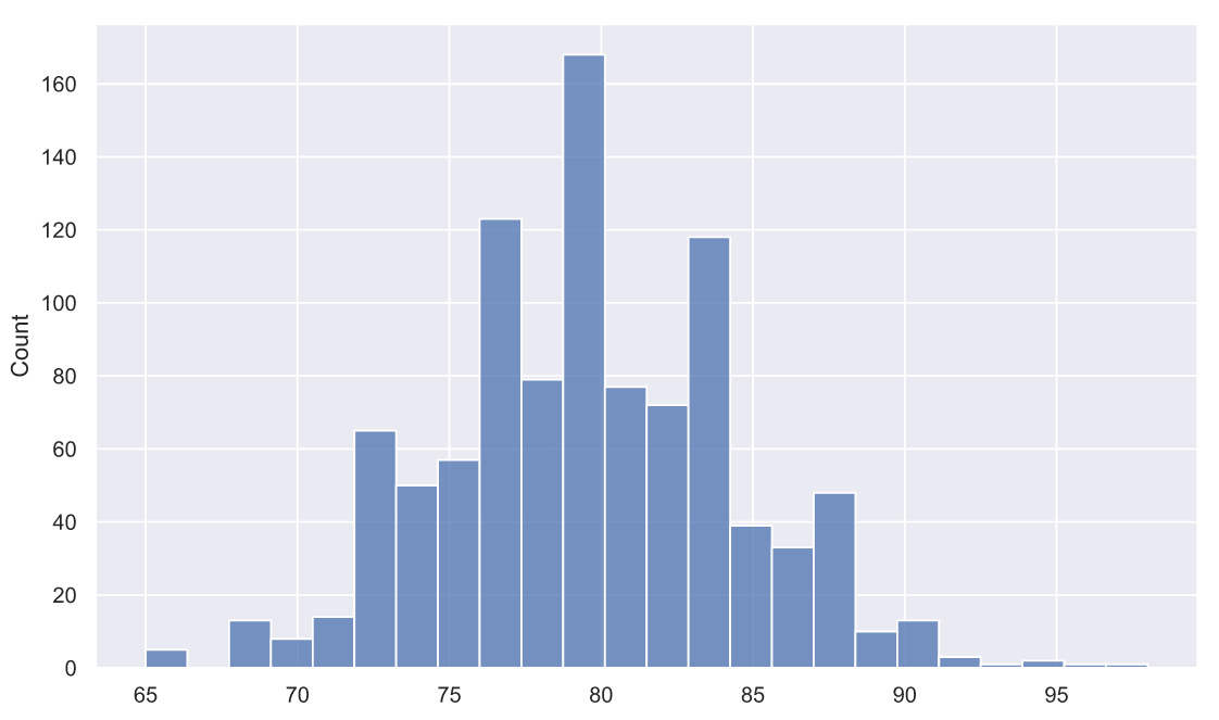
, , . 80 5 . , , , , , - .
, . , - . , - , ? - . , 10 , :
![[89, 99, 93, 84, 79, 61, 82, 81, 87, 82]](https://habrastorage.org/getpro/habr/upload_files/111/47c/b45/11147cb4509f3d49e1c731d87a8b657b.svg)
Z- :

 - ,
- , 
 ,
,  - . :
- . :
sample = np.array([89,99,93,84,79,61,82,81,87,82])
sample.mean()
83.7
Z-:
z = 10**0.5*(sample.mean()-80)/5
z
2.340085468524603
p-value:
1 - (stats.norm.cdf(z) - stats.norm.cdf(-z))
0.019279327322753836
, , : Z- 0 2 , .. 10 , , , 0.02. , 10 , ""  , , 10 "" 83.7 2%. , , , , . .
- 10 , , :
sample.std(ddof=1)
10.055954565441423
ddof std
 , ,
, ,  , . :
, . :

, ,  . -
. - 
 ,
, 
 .
. 
 ? ,
? , 
 -
-  ,
,  .
.  , - .
, - .
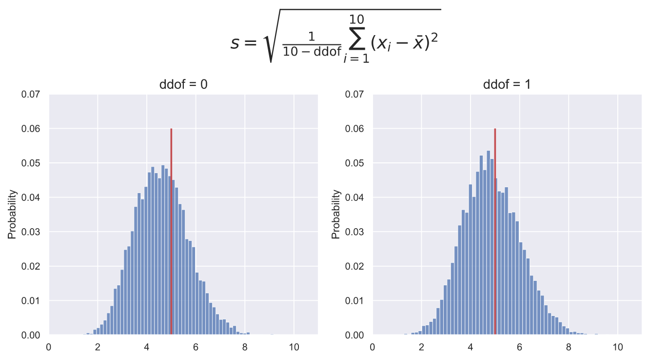
, std() NumPy ddof, 0, std() , , ddof=1. . , 10000 10  , , ddof=0 . ddof=1 , - , ddof=0:
fig, ax = plt.subplots(nrows=1, ncols=2, figsize = (12, 5))
for i in [0, 1]:
deviations = np.std(stats.norm.rvs(80, 5, (10000, 10)), axis=1, ddof=i)
sns.histplot(x=deviations ,stat='probability', ax=ax[i])
ax[i].vlines(5, 0, 0.06, color='r', lw=2)
ax[i].set_title('ddof = ' + str(i), fontsize = 15)
ax[i].set_ylim(0, 0.07)
ax[i].set_xlim(0, 11)
fig.suptitle(r'$s={\sqrt {{\frac {1}{10 - \mathrm{ddof}}}\sum _{i=1}^{10}\left(x_{i}-{\bar {x}}\right)^{2}}}$',
fontsize = 20, y=1.15);
, Z-? , - , . 5000 10 ,  :
:
deviations = np.std(stats.norm.rvs(80, 5, (5000, 10)), axis=1, ddof=1)
sns.histplot(x=deviations ,stat='probability');

, , 10- . . , , 10 2%, , ( ) 10 0. , , : 10- , .
, , , : - , - , . , ""  , Z- p-value 10- :
z = 10**0.5*(sample.mean()-80)/10
p = 1 - (stats.norm.cdf(z) - stats.norm.cdf(-z))
print(f'z = {z:.3}')
print(f'p-value = {p:.4}')
z = 1.17
p-value = 0.242
,  , , , .. ,
  , . 2%, 25%. , -
 .
.
, ? ! , : (, , - )

T-, Z- ,  ,
,  . 10000
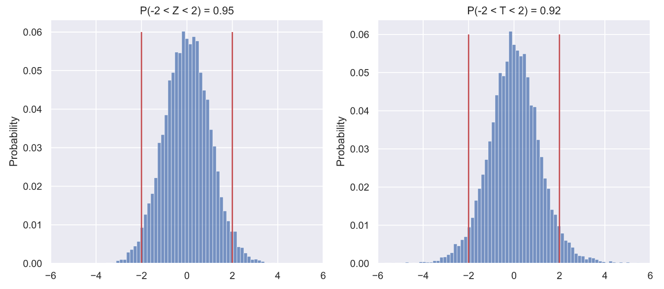
  , Z- T-, :
fig, ax = plt.subplots(nrows=1, ncols=2, figsize = (12, 5))
N = 10000
samples = stats.norm.rvs(80, 5, (N, 10))
statistics = [lambda x: 10**0.5*(np.mean(x, axis=1) - 80)/5,
lambda x: 10**0.5*(np.mean(x, axis=1) - 80)/np.std(x, axis=1, ddof=1)]
title = 'ZT'
bins = np.linspace(-6, 6, 80, endpoint=True)
for i in range(2):
values = statistics[i](samples)
sns.histplot(x=values ,stat='probability', bins=bins, ax=ax[i])
p = values[(values > -2)&(values < 2)].size/N
ax[i].set_title('P(-2 < {} < 2) = {:.3}'.format(title[i], p))
ax[i].set_xlim(-6, 6)
ax[i].vlines([-2, 2], 0, 0.06, color='r');
- :
import matplotlib.animation as animation
fig, axes = plt.subplots(nrows=1, ncols=2, figsize = (18, 8))
def animate(i):
for ax in axes:
ax.clear()
N = 10000
samples = stats.norm.rvs(80, 5, (N, 10))
statistics = [lambda x: 10**0.5*(np.mean(x, axis=1) - 80)/5,
lambda x: 10**0.5*(np.mean(x, axis=1) - 80)/np.std(x, axis=1, ddof=1)]
title = 'ZT'
bins = np.linspace(-6, 6, 80, endpoint=True)
for j in range(2):
values = statistics[j](samples)
sns.histplot(x=values ,stat='probability', bins=bins, ax=axes[j])
p = values[(values > -2)&(values < 2)].size/N
axes[j].set_title(r'$P(-2\sigma < {} < 2\sigma) = {:.3}$'.format(title[j], p))
axes[j].set_xlim(-6, 6)
axes[j].set_ylim(0, 0.07)
axes[j].vlines([-2, 2], 0, 0.06, color='r')
return axes
dist_animation = animation.FuncAnimation(fig,
animate,
frames=np.arange(7),
interval = 200,
repeat = False)
dist_animation.save('statistics_dist.gif',
writer='imagemagick',
fps=1)
, , . ? -, , . , , ? , , 
![[-2 \ sigma; 2 \ sigma]](https://habrastorage.org/getpro/habr/upload_files/f0d/a1c/cfd/f0da1ccfdb352631a44937d502801011.svg) 95.5% . Z- , T- , 92-93% . , , - , :
95.5% . Z- , T- , 92-93% . , , - , :
statistics = [lambda x: 10**0.5*(np.mean(x, axis=1) - 80)/5,
lambda x: 10**0.5*(np.mean(x, axis=1) - 80)/np.std(x, axis=1, ddof=1)]
quantity = 50
N=10000
result = []
for i in range(quantity):
samples = stats.norm.rvs(80, 5, (N, 10))
Z = statistics[0](samples)
p_z = Z[(Z > -2)&((Z < 2))].size/N
T = statistics[1](samples)
p_t = T[(T > -2)&((T < 2))].size/N
result.append([p_z, p_t])
result = np.array(result)
fig, ax = plt.subplots()
line1, line2 = ax.plot(np.arange(quantity), result)
ax.legend([line1, line2],
[r'$P(-2\sigma < {} < 2\sigma)$'.format(i) for i in 'ZT'])
ax.hlines(result.mean(axis=0), 0, 50, color='0.6');
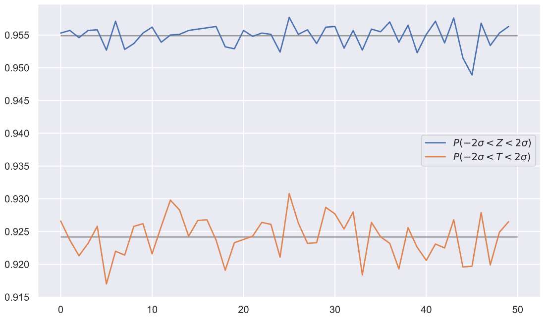
50 . , , , , . ? , ! Z- T- , . , T- ? , - . , , - , , , . , . , - , , 
 .
.
Z-,  ,
,  - . 10000
  10 , :
# ,
# svg png:
#%config InlineBackend.figure_format = 'png'
N = 10000
samples = stats.norm.rvs(80, 5, (N, 10))
means = samples.mean(axis=1)
deviations = samples.std(ddof=1, axis=1)
T = statistics[1](samples)
P = (T > -2)&((T < 2))
fig, ax = plt.subplots()
ax.scatter(means[P], deviations[P], c='b', alpha=0.7,
label=r'$\left | T \right | < 2\sigma$')
ax.scatter(means[~P], deviations[~P], c='r', alpha=0.7,
label=r'$\left | T \right | > 2\sigma$')
mean_x = np.linspace(75, 85, 300)
s = np.abs(10**0.5*(mean_x - 80)/2)
ax.plot(mean_x, s, color='k',
label=r'$\frac{\sqrt{n}(\bar{x}-\mu)}{2}$')
ax.legend(loc = 'upper right', fontsize = 15)
ax.set_title(' \n ',
fontsize=15)
ax.set_xlabel(r' ($\bar{x}$)',
fontsize=15)
ax.set_ylabel(r' ($s$)',
fontsize=15);
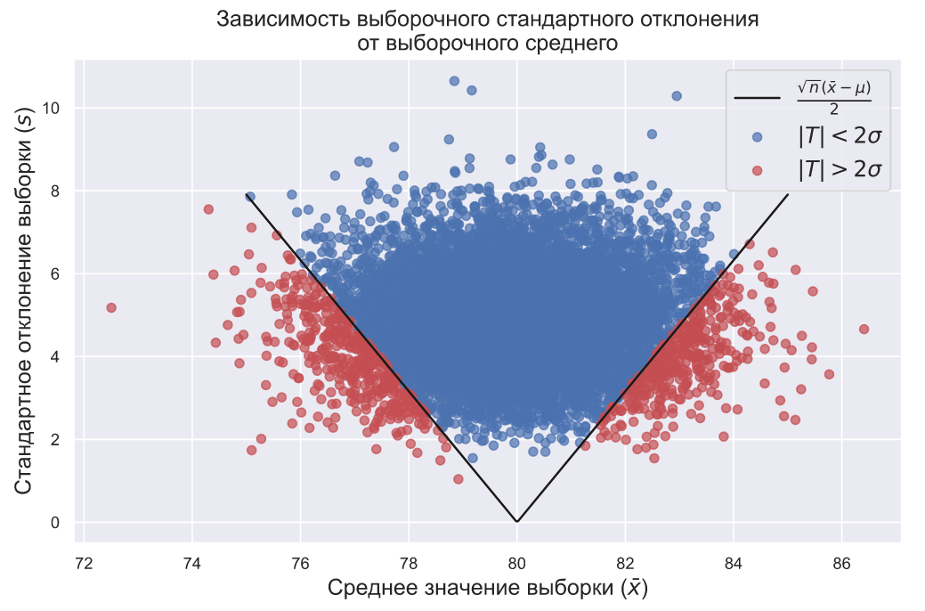
, . , , 
 , .. . , ,
  ,
, 
 . , ( ) , :

,  , .. , , ,
  ,
,  :
:

, ![[-2\sigma; 2\sigma]](https://habrastorage.org/getpro/habr/upload_files/bea/828/453/bea828453e4b32cb920e5d40a188262d.svg) , , 92,5% .
, , 92,5% .
? , . , ( ) 100- . , , ( ). 10- 82- , 2- . , , .  , , ..
  ? Z-:
? Z-:

 p-value:
z = 10**0.5*(82-80)/2
p = 1 - (stats.norm.cdf(z) - stats.norm.cdf(-z))
print(f'p-value = {p:.2}')
p-value = 0.0016
10 82- 2%.  . ,
. ,  , , , .
, , , . (  ) (
) (  ).
).
10 . 82 , , , 9- . ? :
z = 10**0.5*(82-80)/9
p = 1 - (stats.norm.cdf(z) - stats.norm.cdf(-z))
print(f'p-value = {p:.2}')
p-value = 0.48
10 

 . , , - .
, , . :
import matplotlib.animation as animation
fig, ax = plt.subplots(figsize = (15, 9))
def animate(i):
ax.clear()
N = 10000
samples = stats.norm.rvs(80, 5, (N, i))
means = samples.mean(axis=1)
deviations = samples.std(ddof=1, axis=1)
T = i**0.5*(np.mean(samples, axis=1) - 80)/np.std(samples, axis=1, ddof=1)
P = (T > -2)&((T < 2))
prob = T[P].size/N
ax.set_title(r' $s$ $\bar{x}$ $n = $' + r'${}$'.format(i),
fontsize = 20)
ax.scatter(means[P], deviations[P], c='b', alpha=0.7,
label=r'$\left | T \right | < 2\sigma$')
ax.scatter(means[~P], deviations[~P], c='r', alpha=0.7,
label=r'$\left | T \right | > 2\sigma$')
mean_x = np.linspace(75, 85, 300)
s = np.abs(i**0.5*(mean_x - 80)/2)
ax.plot(mean_x, s, color='k',
label=r'$\frac{\sqrt{n}(\bar{x}-\mu)}{2}$')
ax.legend(loc = 'upper right', fontsize = 15)
ax.set_xlim(70, 90)
ax.set_ylim(0, 10)
ax.set_xlabel(r' ($\bar{x}$)',
fontsize='20')
ax.set_ylabel(r' ($s$)',
fontsize='20')
return ax
dist_animation = animation.FuncAnimation(fig,
animate,
frames=np.arange(5, 21),
interval = 200,
repeat = False)
dist_animation.save('sigma_rel.gif',
writer='imagemagick',
fps=3)

, 


 , .
, .  Z-,
Z-,  .
.
! , ? - , , . , , 10- :
![[89,99,93,84,79,61,82,81,87,82]](https://habrastorage.org/getpro/habr/upload_files/e5d/05a/011/e5d05a011425a07da6167192fdea7c18.svg)
 ,
,  , , , , ,
  . Z-, T-, Z- ,
 . , -
. , -  ,
,  - ?
- ?  ?: ,
?: ,  ,
,  ,
, 
 ?
?
, . , - . ,  , , , 10 , 10 . ,
  . , - , .
:  ,
,  ,
, 
 . , ,
. , , 
 :
:
N = 10000
sigma = np.linspace(5, 20, 151)
prob = []
for i in sigma:
p = []
for j in range(10):
samples = stats.norm.rvs(80, i, (N, 10))
means = samples.mean(axis=1)
deviations = samples.std(ddof=1, axis=1)
p_m = means[(means >= 83) & (means <= 84)].size/N
p_d = deviations[(deviations >= 9.5) & (deviations <= 10.5)].size/N
p.append(p_m*p_d)
prob.append(sum(p)/len(p))
prob = np.array(prob)
fig, ax = plt.subplots()
ax.plot(sigma, prob)
ax.set_xlabel(r' ($\sigma$)',
fontsize=20)
ax.set_ylabel('',
fontsize=20);
,  . , ,
. , ,  ,
,  . - , , , , . .
T-?
, - - . 1% , - . , , . , - -. ?
- ! , - , "" t-. , , , . , , 1943 , 50% . , - .
, "" . , ( !) , "" , :

t-, . , , "", , , , , - . " ", "t-" , .
:

" " .  , ..
, ..  ,
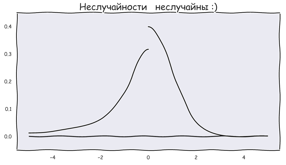
,  , .. , . - , :

, :
import matplotlib.animation as animation
fig, ax = plt.subplots(figsize = (15, 9))
def animate(i):
ax.clear()
N = 15000
x = np.linspace(-5, 5, 100)
ax.plot(x, stats.norm.pdf(x, 0, 1), color='r')
samples = stats.norm.rvs(0, 1, (N, i))
t = samples[:, 0]/np.sqrt(np.mean(samples[:, 1:]**2, axis=1))
t = t[(t>-5)&(t<5)]
sns.histplot(x=t, bins=np.linspace(-5, 5, 100), stat='density', ax=ax)
ax.set_title(r' $t(n)$ n = ' + str(i), fontsize = 20)
ax.set_xlim(-5, 5)
ax.set_ylim(0, 0.5)
return ax
dist_animation = animation.FuncAnimation(fig,
animate,
frames=np.arange(2, 21),
interval = 200,
repeat = False)
dist_animation.save('t_rel_of_df.gif',
writer='imagemagick',
fps=3)
,  , , ,
, , ,  . , , :

SciPy:
import matplotlib.animation as animation
fig, ax = plt.subplots(figsize = (15, 9))
def animate(i):
ax.clear()
N = 15000
x = np.linspace(-5, 5, 100)
ax.plot(x, stats.norm.pdf(x, 0, 1), color='r')
ax.plot(x, stats.t.pdf(x, df=i))
ax.set_title(r' $t(n)$ n = ' + str(i), fontsize = 20)
ax.set_xlim(-5, 5)
ax.set_ylim(0, 0.45)
return ax
dist_animation = animation.FuncAnimation(fig,
animate,
frames=np.arange(2, 21),
interval = 200,
repeat = False)
dist_animation.save('t_pdf_rel_of_df.gif',
writer='imagemagick',
fps=3)

,  ( df ) . - , ,
  , .
, .
t-
t- SciPy :
sample = np.array([89,99,93,84,79,61,82,81,87,82])
stats.ttest_1samp(sample, 80)
Ttest_1sampResult(statistic=1.163532240174695, pvalue=0.2745321678073461)
:
T = 9**0.5*(sample.mean() -80)/sample.std()
T
1.163532240174695
,  ,
,  ,
,  . , 1 , , , . :
T = 10**0.5*(sample.mean() -80)/sample.std(ddof=1)
T
1.1635322401746953
, t- , p-value? , - , p-value Z-, t-:
t = stats.t(df=9)
fig, ax = plt.subplots()
x = np.linspace(t.ppf(0.001), t.ppf(0.999), 300)
ax.plot(x, t.pdf(x))
ax.hlines(0, x.min(), x.max(), lw=1, color='k')
ax.vlines([-T, T], 0, 0.4, color='g', lw=2)
x_le_T, x_ge_T = x[x<-T], x[x>T]
ax.fill_between(x_le_T, t.pdf(x_le_T), np.zeros(len(x_le_T)), alpha=0.3, color='b')
ax.fill_between(x_ge_T, t.pdf(x_ge_T), np.zeros(len(x_ge_T)), alpha=0.3, color='b')
p = 1 - (t.cdf(T) - t.cdf(-T))
ax.set_title(r'$P(\left | T \right | \geqslant {:.3}) = {:.3}$'.format(T, p));

, p-value 27%, .. , - ,  , p-value , 5 . , , - ,
  , 0.95:

SciPy, interval loc () scale () :
sample_loc = sample.mean()
sample_scale = sample.std(ddof=1)/10**0.5
ci = stats.t.interval(0.95, df=9, loc=sample_loc, scale=sample_scale)
ci
(76.50640345566619, 90.89359654433382)
,  , ,
, , 
![[76.5; 90.9]](https://habrastorage.org/getpro/habr/upload_files/271/4c8/21d/2714c821d6a7a520116d1a2df7c3059c.svg) . , ,
. , ,  , .
, .
, , , ( ). , , t- , t- , t- .
Of course, I would like to insert some gif at the end, but I want to end with the phrase of Herbert Spencer: " The greatest goal of education is not knowledge, but action ", so launch your anacondas and take action ! This is especially true for self-taught people like me.
I press F5 and look forward to your comments!