Python, correlation and regression: part 4

See the previous post here .

Prediction

Finally, we come to one of the most important applications of linear regression: prediction . We trained a model to predict the weight of Olympic swimmers given their height, gender, and year of birth.

9-time Olympic swimming champion Mark Spitz won 7 gold medals at the 1972 Olympics. He was born in 1950 and, according to the Wikipedia website, is 183 cm tall and weighs 73 kg. Let's see what our model predicts in terms of its weight.

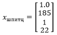
Our multiple regression model requires these values ​​to be provided in matrix form. Each parameter must be passed in the order in which the model learned the features in order to apply the correct coefficient. After the bias, the feature vector should contain height, gender and year of birth in the same units in which the model was trained:

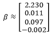
The β  matrix contains the coefficients for each of these features:

The model prediction will be the sum of the products of the coefficients β  and features x  in each row:

, β  xspitz.

, :

β^Tx — 1 × n  n × 1. 1 × 1:

 

:

def predict(coefs, x): 
    ''' '''
    return np.matmul(coefs, x.values) 
      
      

        
        
        
      

    
        
        
        
      
      

        
        
        
      

    
    

def ex_3_29():
    '''   '''
    df = swimmer_data()
    df['_'] = df[''].map({'': 1, '': 0}).astype(int) 
    df[' '] = df[' '].map(str_to_year)
    X = df[[', ', '_', ' ']] 
    X.insert(0, '', 1.0)
    y = df[''].apply(np.log) 
    beta = linear_model(X, y)
    xspitz = pd.Series([1.0, 183, 1, 1950]) #   
    return np.exp( predict(beta, xspitz) )  
      
      

        
        
        
      

    
        
        
        
      
      

        
        
        
      

    
    

84.20713139038605
      
      

        
        
        
      

    
        
        
        
      
      

        
        
        
      

    
    

84.21, 84.21 . 73 . , , .

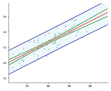
. , , . , , . ŷ  , , μ. , , y  ^.

^{, , , . 95%- – , 95% . , 95%- – , 95%- .}

. , :

ŷ_p — , . t-, n - p, .. . , F-. , , , , , 95%- .

def prediction_interval(x, y, xp):
    '''  '''
    xtx    = np.matmul(x.T, np.asarray(x))
    xtxi   = np.linalg.inv(xtx)  
    xty    = np.matmul(x.T, np.asarray(y)) 
    coefs  = linear_model(x, y) 
    fitted = np.matmul(x, coefs)
    resid  = y - fitted
    rss    = resid.dot(resid)  
    n      = y.shape[0]  # 
    p      = x.shape[1]  # 
    dfe    = n - p 
    mse    = rss / dfe
    se_y   = np.matmul(np.matmul(xp.T, xtxi), xp)
    t_stat = np.sqrt(mse * (1 + se_y))         # t-
    intl   = stats.t.ppf(0.975, dfe) * t_stat   
    yp     = np.matmul(coefs.T, xp)
    return np.array([yp - intl, yp + intl])
      
      

        
        
        
      

    
        
        
        
      
      

        
        
        
      

    
    

t- , .

, se_y



t- t_stat



.

, , :

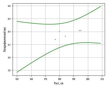
5 , 95%- . , :

def ex_3_30():
    ''' 
            '''
    df = swimmer_data()
    df['_'] = df[''].map({'': 1, '': 0}).astype(int) 
    df[' '] = df[' '].map(str_to_year)
    X = df[[', ', '_', ' ']] 
    X.insert(0, '', 1.0)
    y = df[''].apply(np.log) 
    xspitz = pd.Series([1.0, 183, 1, 1950])  #  .
    return np.exp( prediction_interval(X, y, xspitz) )
      
      

        
        
        
      

    
        
        
        
      
      

        
        
        
      

    
    

array([72.74964444, 97.46908087])
      
      

        
        
        
      

    
        
        
        
      
      

        
        
        
      

    
    

72.7 97.4 ., 73 ., 95%- . .

1950 ., 2012 . , , , . .

, . , , . , , . 1979 ., .

, 1972 . 22- 185 . 79 .

^{— .}

, , .

R², , . , .. , , , - .

β  :

1972 . :

:

def ex_3_32():
    '''    
        '''
    df = swimmer_data()
    df['_'] = df[''].map({'': 1, '': 0}).astype(int) 
    X = df[[', ', '_', '']] 
    X.insert(0, '', 1.0)
    y = df[''].apply(np.log) 

    beta = linear_model(X, y)
    #    
    xspitz = pd.Series([1.0, 185, 1, 22]) 
    return np.exp( predict(beta, xspitz) )
      
      

        
        
        
      

    
        
        
        
      
      

        
        
        
      

    
    

78.46882772630318
      
      

        
        
        
      

    
        
        
        
      
      

        
        
        
      

    
    

78.47, .. 78.47 . , 79 .

   Github.    . 

, . , r  R²  R̅². , ρ .

, Python. , pandas numpy . β, , . , .