See the previous post here .
Regression
While it may be helpful to know that the two variables are correlated, we cannot use this information alone to predict the weight of Olympic swimmers in the presence of height data, or vice versa. When establishing the correlation, we measured the strength and sign of the connection, but not the slope, i.e. slope. To generate a prediction, you need to know the expected rate of change in one variable for a given unit change in another.
We would like to derive an equation that relates the specific value of one variable, the so-called independent variable, to the expected value of another, dependent variable. For example, if our linear equation predicts weight for a given height, the growth is our independent variable , and weight - dependent .
The lines described by these equations are called regression lines . This Term was coined by the 19th century British polymath Sir Francis Galton. He and his student Carl Pearson, who derived the correlation coefficient, developed a large number of methods for studying linear relationships in the 19th century, which collectively became known as regression analysis methods.
Recall that correlation does not imply causation, and the terms “dependent” and “independent” do not mean any implicit causation. They are just names for input and output math values. A classic example is the extremely positive correlation between the number of fire trucks sent to extinguish a fire and the damage caused by the fire. Of course, sending fire trucks to extinguish a fire does not in itself cause damage. No one would advise reducing the number of vehicles sent to extinguish a fire as a way to reduce damage. In such situations, we must look for an additional variable that would be causally related to other variables and explain the correlation between them. In this example, it could be the size of the fire... These underlying causes are called confounding variables because they distort our ability to determine the relationship between dependent variables.
Linear Equations
The two variables, which we can denote as x and y , can be strictly or loosely related to each other. The simplest relationship between the independent variable x and the dependent variable y is straightforward, which is expressed by the following formula:

a b . a , b — , . , a = 32 b = 1.8. a b, :

10° x 10:

, , 10° 50°F, . Python pandas, , :
'''       '''
celsius_to_fahrenheit = lambda x: 32 + (x * 1.8)

def ex_3_11():
    '''    '''
    df = pd.DataFrame({'C':s, 'F':s.map(celsius_to_fahrenheit)})
    df.plot('C', 'F', legend=False, grid=True)
    plt.xlabel(' ')
    plt.ylabel(' ')
    plt.show()
:
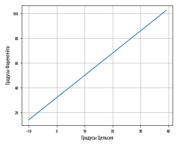
, 0 32 . a — y, x 0.
b; 2. , . , , .
, , . y x. , , , , :

, ε — , , a b x y. y — ŷ, — :

. - , , , . , , , ( ).
a b , x , . , , , x y.
, , , , , . , , .
, , , . , , , .
, , . , . Ordinary Least Squares (OLS), :

, , , . , , , :
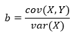
(a) — , X Y:

a b — , .
covariance
, variance
mean
, . :
def slope(xs, ys):
    '''   ( )'''
    return xs.cov(ys) / xs.var()

def intercept(xs, ys):
     '''   (  Y)'''
   return ys.mean() - (xs.mean() * slope(xs, ys))

def ex_3_12():
    '''    ( )
            '''
    df = swimmer_data()
    X  = df[', ']
    y  = df[''].apply(np.log)
    a  = intercept(X, y)
    b  = slope(X, y)
    print(': %f, : %f' % (a,b))
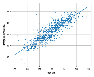
: 1.691033, : 0.014296
0.0143 1.6910.
— ( ), () . np.exp
, np.log
. , 5.42 . , , .
, y x. , 1.014 . . , , , .
regression_line
x, ŷ a b.
'''  '''
regression_line = lambda a, b: lambda x: a + (b * x)  #  fn(a,b)(x)

def ex_3_13():
    '''
            '''
    df = swimmer_data()
    X  = df[', '].apply( jitter(0.5) )
    y  = df[''].apply(np.log)
    a, b = intercept(X, y), slope(X, y)
    ax = pd.DataFrame(np.array([X, y]).T).plot.scatter(0, 1, s=7)
    s  = pd.Series(range(150,210))
    df = pd.DataFrame( {0:s, 1:s.map(regression_line(a, b))} )
    df.plot(0, 1, legend=False, grid=True, ax=ax)
    plt.xlabel(', .')
    plt.ylabel(' ')
    plt.show()
regression_line
x, a + bx.
, , ŷ y.
def residuals(a, b, xs, ys):
    ''' '''
    estimate = regression_line(a, b)     #
    return pd.Series( map(lambda x, y: y - estimate(x), xs, ys) )

constantly = lambda x: 0

def ex_3_14():
    '''        '''
    df = swimmer_data()
    X  = df[', '].apply( jitter(0.5) )
    y  = df[''].apply(np.log)
    a, b = intercept(X, y), slope(X, y)
    y  = residuals(a, b, X, y)
    ax = pd.DataFrame(np.array([X, y]).T).plot.scatter(0, 1, s=12)
    s  = pd.Series(range(150,210))
    df = pd.DataFrame( {0:s, 1:s.map(constantly)} )
    df.plot(0, 1, legend=False, grid=True, ax=ax)
    plt.xlabel(', .')
    plt.ylabel('')
    plt.show()
— , Y X. , :
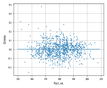
, , -, , . , . , , .
, , , . , . , , . , .
, . . , , , .. . , , , .
. , , , , .
R-
, , .. , . R2, R-, 0 1 . .
, R2 1, Y X. R2 :
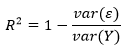
var(ε) — var(Y) — Y. , - . , . var(Y), .. .
, , a + bx. .
var(ε)/var(Y) — , . . , . R2 — , .
r, R2 , . , .
R2 . — , R2. R2 .
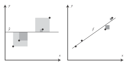
, , , , f. , y. R2 y:
def r_squared(a, b, xs, ys):
    '''   (R-)'''
    r_var = residuals(a, b, xs, ys).var()
    y_var = ys.var()
    return 1 - (r_var / y_var)

def ex_3_15():
    '''  R-
            '''
    df = swimmer_data()
    X  = df[', '].apply( jitter(0.5) )
    y  = df[''].apply(np.log)
    a, b = intercept(X, y), slope(X, y)
    return r_squared(a, b, X, y)
0.75268223613272323
0.753. , 75% , 2012 ., .
( ), R2 r :
r , Y X, R2 0.52, .. 0.25.
, . , . .
. , , β (), :

- , β1 = a β2 = b , x1 1, β1 — , , x1 () , .
β, , :

x1 xn , y. β1 βn , .
, : , , , . , , .
, x. pandas, , : .
The source code examples for this post are in my Github repo . All source data is taken from the repository of the author of the book.
The topic of the next post, post # 3 , will be matrix operations, normal equation and collinearity.