The more I get to know people, the more I like my dog.
-Mark Twain
In the previous series of posts for beginners of remixes book Henry Garner « Clojure's data research » (Clojure for Data Science) in Python we have reviewed methods to describe the sample in terms of the summary statistics and statistical inference methods are population parameters. This analysis tells us something about the population in general and about the sample in particular, but it does not allow us to make very precise statements about their individual elements. This is because reducing the data to just two statistics - the mean and the standard deviation - loses a huge amount of information.
We often need to go further and establish a relationship between two or more variables, or predict one variable in the presence of another. And that brings us to the topic of this 5-post series - exploring correlation and regression. Correlation deals with the strength and directionality of a relationship between two or more variables. Regression determines the nature of this relationship and allows predictions to be made based on it.
This series of posts will cover linear regression . Given a sample of data, our model will learn a linear equation that allows it to make predictions about new, previously unseen data. To do this, we will go back to the pandas library and examine the relationship between height and weight in Olympic athletes. We will introduce the concept of matrices and show you how to manage them using the pandas library.
About data
This series of posts uses data courtesy of Guardian News and Media Ltd. on athletes who competed in the 2012 London Olympics. This data was originally taken from the blog of the Guardian newspaper.
Data survey
When faced with a new dataset, the first task is to survey it in order to understand what exactly it contains.
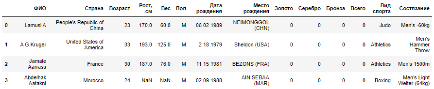
The all-london-2012-athletes.tsv file is fairly small. We can explore the data using pandas, as we did in the first series of posts " Python, Data Exploration and Choices, " using the function read_csv
:
def load_data():
    return pd.read_csv('data/ch03/all-london-2012-athletes-ru.tsv', '\t')

def ex_3_1():
    '''
           2012 .'''
    return load_data()
If you run this example in the Python interpreter console or in a Jupyter notebook, you should see the following output:
|
|
|
|
( , ) :
,
,
, .
, .
«» «»
( )
,
,
,
, , , . , .
2012 . . , , :
def ex_3_2():
    '''
          '''
    df = load_data()
    df[', '].hist(bins=20)
    plt.xlabel(', .')
    plt.ylabel('')
    plt.show()
:
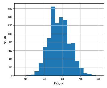
, . 177 . :
def ex_3_3():
    '''    '''
    df = load_data()
    df[''].hist(bins=20)
    plt.xlabel('')
    plt.ylabel('')
    plt.show()
:
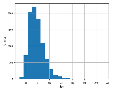
. , , , - . pandas skew
:
def ex_3_4():
    '''   '''
    df = load_data()
    swimmers = df[ df[' '] == 'Swimming']
    return swimmers[''].skew()
0.23441459903001483
, numpy np.log
:
def ex_3_5():
    '''

       '''
    df = load_data()
    df[''].apply(np.log).hist(bins=20)
    plt.xlabel(' ')
    plt.ylabel('')
    plt.show()
:
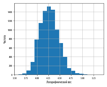
. , .
— , . . , .
, () . , , . 10 e, , 2.718. numpy np.log
np.exp
e. loge , ln, - , .
, . , c 1931 . , , . , , .
, , , , , .
, , , Wolfram MathWorld, .
, . , , .
, . , , :
def swimmer_data():
    '''       '''
    df = load_data()
    return df[df[' '] == 'Swimming'].dropna()

def ex_3_6():
    '''     '''
    df = swimmer_data()
    xs = df[', ']
    ys = df[''].apply( np.log )
    pd.DataFrame(np.array([xs,ys]).T).plot.scatter(0, 1, s=12, grid=True)
    plt.xlabel(', .')
    plt.ylabel(' ')
    plt.show()
:

, . , . :

, , , . , , , . , , , - ( . . ). , , , , . ( ) , , , , , . .
, , 180 , 179.5 180.5 , 80 79.5 80.5 . , -0.5 0.5 (, c , ):
def jitter(limit):
    '''  (   )'''
    return lambda x: random.uniform(-limit, limit) + x

def ex_3_7():
    '''       '''
    df = swimmer_data()
    xs = df[', '].apply(jitter(0.5))
    ys = df[''].apply(jitter(0.5)).apply(np.log)
    pd.DataFrame(np.array([xs,ys]).T).plot.scatter(0, 1, s=12, grid=True)
    plt.xlabel(', .')
    plt.ylabel(' ')
    plt.show()
:

, — , , , .
. .
, X Y, :


xi — X i, yi — Y i, x̅ — X, y̅ — Y. X Y , : , — , , . , , , , . .
:

Python :
def covariance(xs, ys):
    '''  (, .. n-1)'''
    dx = xs - xs.mean()
    dy = ys - ys.mean()
    return (dx * dy).sum() / (dx.count() - 1)
, pandas cov
:
df[', '].cov(df[''])
1.3559273321696459
1.356, . .
. , . -1 +1. .
, . standard score, z- — , . , , — . , .
r , dxi dyi :

X Y , , σx σy — X Y:

, , r.
. :
def variance(xs):
    ''' ,
          n <= 30'''
    x_hat = xs.mean()
    n = xs.count()
    n = n - 1 if n in range( 1, 30 ) else n
    return sum((xs - x_hat) ** 2) / n

def standard_deviation(xs):
    '''  '''
    return np.sqrt(variance(xs))

def correlation(xs, ys):
    ''' '''
    return covariance(xs, ys) / (standard_deviation(xs) *
                                 standard_deviation(ys))
pandas corr
:
df[', '].corr(df[''])
, r . r -1.0 1.0, .
, r = 0, , . . , , r :

, , y = 0. r 0, . ; y . .
:
def ex_3_8():
    '''   pandas
            '''
    df = swimmer_data()
    return df[', '].corr( df[''].apply(np.log))
0.86748249283924894
0.867, , , .
r ρ
, . ; , : . r, ρ ().
, , , , . , . , , , -.
— , , — . , r, ρ, :
r
, , , . , , , . , .
, , (, , ) . , , .
, , :


H0 - , . , , .
H1 - , . , , . , .
r :

, r (, ρ ), , , .
t- t-:

df — . n - 2, n — . , :

t- 102.21. p- t-. scipy () t- stats.t.cdf
, (1-cdf) stats.t.sf
. p- . 2, :
def t_statistic(xs, ys):
    ''' t-'''
    r = xs.corr(ys)  #  , correlation(xs, ys)
    df = xs.count() - 2
    return r * np.sqrt(df / 1 - r ** 2)

def ex_3_9():
    '''  t-'''
    df = swimmer_data()
    xs = df[', ']
    ys = df[''].apply(np.log)
    t_value = t_statistic(xs, ys)
    df = xs.count() - 2
    p = 2 * stats.t.sf(t_value, df)  #
    return {'t-':t_value, 'p-':p}
{'p-': 1.8980236317815443e-106, 't-': 25.384018200627057}
P- , 0, , , , . .
, , , , , , , , , ρ, . , r ( %), ρ .
, . r 1, r r .

r- ρ, 0.6.
, z- r . , , .
z- :

z :

, r z z-, SEz r.
SEz, , . 1.96, , 95% . , 1.96 r ρ 95%- .

, scipy stats.norm.ppf
. , .
, , , .. 2.5%, , 95%- . 100%. , 95% , 97.5%:
def critical_value(confidence, ntails): #
    '''

          '''
    lookup = 1 - ((1 - confidence) / ntails)
    return stats.norm.ppf(lookup, 0, 1)  # mu=0, sigma=1

critical_value(0.95, 2)
1.959963984540054
95%- z- ρ :

zr SEz, :

r=0.867 n=859 1.137 1.722. z- r-, z-:

:
def z_to_r(z):
    ''' z-   r-'''
    return (np.exp(z*2) - 1) / (np.exp(z*2) + 1)

def r_confidence_interval(crit, xs, ys):
    '''
           '''
    r   = xs.corr(ys)
    n   = xs.count()
    zr  = 0.5 * np.log((1 + r) / (1 - r))
    sez = 1 / np.sqrt(n - 3)
    return (z_to_r(zr - (crit * sez))), (z_to_r(zr + (crit * sez)))

def ex_3_10():
    '''
            '''
    df = swimmer_data()
    X = df[', ']
    y = df[''].apply(np.log)
    interval = r_confidence_interval(1.96, X, y)
    print('  (95%):', interval)
(95%): (0.8499088588880347, 0.8831284878884087)
95%- ρ, 0.850 0.883. , .
The source code examples for this post are in my Github repo . All source data are taken from the repository of the author of the book.
In the next post, post # 2 , the topic of the series itself will be considered - regression and techniques for assessing its quality.