I don’t know about you, but statistics were not easy for me. Moreover, "was given" - this is still loudly said. Yes, it turned out that you can go for a rather long time on training manuals, somehow delving into the meaning of the four-story formulas, and sometimes not even understanding the results, but still go. To go and not get any pleasure - everything seems to be clear, but the feeling that you are "not quite in the subject" still does not leave. For some time I tried to read books on R and not that it would be completely unsuccessful, but not "fire" either. I found the coolest book "Statistics for All" by Sarah Boslaf, read it ... still there were some nuances, the meaning of which is not fully understood.
In general, as you guessed it, this article is from the series "I try to explain on my fingers to figure it out myself." So if you are not indifferent to statistics, then please, under cat.
, , . , :
" " . . , . . ;
" " . . . , , " ". , - , " " . , , - - . :
" " . . . . "", . .
" " . , , , . , , , . , . , , . , , . .
, ", , , ", , , "".
(- , ) " - ". NumPy, matplotlib, seaborn SciPy - . , .
... , - :
import numpy as np
from scipy import stats
import matplotlib.pyplot as plt
#import seaborn as sns
from pylab import rcParams
#sns.set()
rcParams['figure.figsize'] = 10, 6
%config InlineBackend.figure_format = 'svg'
np.random.seed(42)
, , , , , . :
norm_rv = stats.norm(loc=30, scale=5)
samples = np.trunc(norm_rv.rvs(365))
samples[:30]
array([32., 29., 33., 37., 28., 28., 37., 33., 27., 32., 27., 27., 31.,
20., 21., 27., 24., 31., 25., 22., 37., 28., 30., 22., 27., 30.,
24., 31., 26., 28.])
:
samples.mean(), samples.std()
(29.52054794520548, 4.77410133275075)
, -  .
.
, , :
sns.histplot(x=samples, discrete=True);

, , 
 . , , ? ? , , :
norm_rv = stats.norm(loc=30, scale=5)
beta_rv = stats.beta(a=5, b=5, loc=14, scale=32)
gamma_rv = stats.gamma(a = 20, loc = 7, scale=1.2)
tri_rv = stats.triang(c=0.5, loc=17, scale=26)
x = np.linspace(10, 50, 300)
sns.lineplot(x = x, y = norm_rv.pdf(x), color='r', label='norm')
sns.lineplot(x = x, y = beta_rv.pdf(x), color='g', label='beta')
sns.lineplot(x = x, y = gamma_rv.pdf(x), color='k', label='gamma')
sns.lineplot(x = x, y = tri_rv.pdf(x), color='b', label='triang')
sns.histplot(x=samples, discrete=True, stat='probability',
alpha=0.2);

?
, :
;
- ;
;
;
;
, .
, , ( , - . ?). , , , .. . ,  , . , :
unif_rv = stats.uniform(loc=0, scale=4)
unif_rv.rvs()
0.8943833540778106
, - -- :
unif_rv.rvs(size=3)
array([3.85289016, 0.0486179 , 3.87951531])
, 15 , . , :
- , - .. ;
, , , - .. ;
, , , , - - .. .
15 :  , , ,
, , ,  :
:

 , -
, -  ? 10 :
Y_samples = [unif_rv.rvs(size=15).sum() for i in range(10000)]
sns.histplot(x=Y_samples);

, ? , , : .
, , :
. , ;
- . - ;
. ;
. , ;
. ?;
, . , .
,  , . , , :

:

 ? , . , 365- , , , .
Z-
, . , . ,  , , 40 , 35 .
? , ? , , ,  , 27, 31, 35 , 23 38 . , 365 , 20 45 .
  , , - 25 35 . , :
N = 5000
t_data = norm_rv.rvs(N)
t_data[(25 < t_data) & (t_data < 35)].size/N
0.7008
- 25 35 . 40 ?
t_data[t_data > 40].size/N
0.0248
40 . 40 . , :
0.02**3
8.000000000000001e-06
, - . Z-.
Z- :

 - , .. -
  , ,
, , 
 . , .. , 30 5 . Z- :

? , . Z-? "":
fig, ax = plt.subplots()
x = np.linspace(norm_rv.ppf(0.001), norm_rv.ppf(0.999), 200)
ax.vlines(40.5, 0, 0.1, color='k', lw=2)
sns.lineplot(x=x, y=norm_rv.pdf(x), color='r', lw=3)
sns.histplot(x=samples, stat='probability', discrete=True);

samples, , . . 40 . , . - , .. , , 5000 , , :
np.random.seed(42)
N = 10000
values = np.trunc(norm_rv.rvs(N))
fig, ax = plt.subplots()
v_le_41 = np.histogram(values, np.arange(9.5, 41.5))
v_ge_40 = np.histogram(values, np.arange(40.5, 51.5))
ax.bar(np.arange(10, 41), v_le_41[0]/N, color='0.8')
ax.bar(np.arange(41, 51), v_ge_40[0]/N)
p = np.sum(v_ge_40[0]/N)
ax.set_title('P(Y>40min) = {:.3}'.format(p))
ax.vlines(40.5, 0, 0.08, color='k', lw=1);
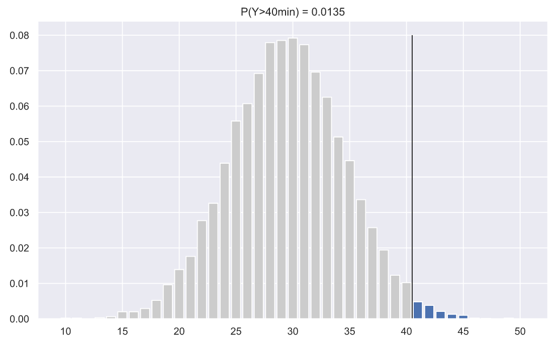
- . , , . , , , . , , 40 :
fig, ax = plt.subplots()
x = np.linspace(norm_rv.ppf(0.0001), norm_rv.ppf(0.9999), 300)
ax.plot(x, norm_rv.pdf(x))
ax.fill_between(x[x>41], norm_rv.pdf(x[x>41]), np.zeros(len(x[x>41])))
p = 1 - norm_rv.cdf(41)
ax.set_title('P(Y>40min) = {:.3}'.format(p))
ax.hlines(0, 10, 50, lw=1, color='k')
ax.vlines(41, 0, 0.08, color='k', lw=1);

. , , - , "", - , . , - , . 40 , .. 41, 42, 43 .. . 41.0. , SciPy , , - . , , - , : , , .. , Z-.
, - 
 . 99 143 , ? , , :
fig, ax = plt.subplots(nrows=1, ncols=2, figsize = (12, 5))
nrv_hobbit = stats.norm(91, 8)
nrv_gnome = stats.norm(134, 6)
for i, (func, h) in enumerate(zip((nrv_hobbit, nrv_gnome), (99, 143))):
x = np.linspace(func.ppf(0.0001), func.ppf(0.9999), 300)
ax[i].plot(x, func.pdf(x))
ax[i].fill_between(x[x>h], func.pdf(x[x>h]), np.zeros(len(x[x>h])))
p = 1 - func.cdf(h)
ax[i].set_title('P(H > {} ) = {:.3}'.format(h, p))
ax[i].hlines(0, func.ppf(0.0001), func.ppf(0.9999), lw=1, color='k')
ax[i].vlines(h, 0, func.pdf(h), color='k', lw=2)
ax[i].set_ylim(0, 0.07)
fig.suptitle(' , ', fontsize = 20);

, , , ( ), . , . "".
Z-:

fig, ax = plt.subplots()
N_rv = stats.norm()
x = np.linspace(N_rv.ppf(0.0001), N_rv.ppf(0.9999), 300)
ax.plot(x, N_rv.pdf(x))
ax.hlines(0, -4, 4, lw=1, color='k')
ax.vlines(1, 0, 0.4, color='r', lw=2, label='')
ax.vlines(1.5, 0, 0.4, color='g', lw=2, label='')
ax.legend();

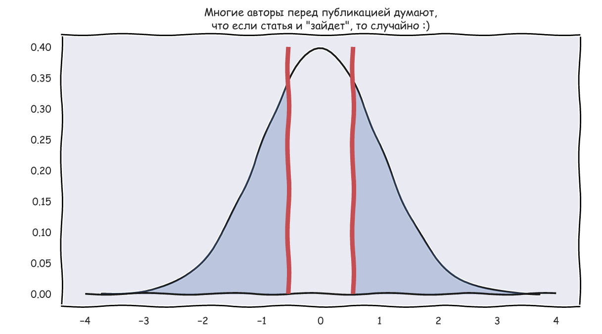
Z- , "", ..  , Z- . , , , Z- . :

, .
Z- "" , Z- . :

, : , , ; , Z- . Z-, , Z- .
, - - . , . , , Z- - () , . . , , , . - .
Z-
, . Z- 40 :

, , :
fig, ax = plt.subplots()
N_rv = stats.norm()
x = np.linspace(N_rv.ppf(0.0001), N_rv.ppf(0.9999), 300)
ax.plot(x, N_rv.pdf(x))
ax.hlines(0, -4, 4, lw=1, color='k')
ax.vlines(2, 0, 0.4, color='g', lw=2);

 , . , , . , - !
, - . 365- , , .. ,  . . , , , . 5000 :
sns.histplot(np.trunc(norm_rv.rvs(size=(N, 3))).mean(axis=1),
bins=np.arange(19, 42));

, 40 - . :
;
- , .. - , .
Z- (Z = 2), ( ) :
1 - N_rv.cdf(2)
0.02275013194817921
, 40 :
(1 - N_rv.cdf(2))**3
1.1774751750476762e-05
Z-, - Z-:

 - ,
- , 
 ,
,  - .
- .
35 , Z- :

Z-, Z- , . , ,

[25; 35] . :
N = 10000
means = np.trunc(norm_rv.rvs(size=(N, 3))).mean(axis=1)
means[(means>=25)&(means<=35)].size/N
0.9241
N = 10000
fig, ax = plt.subplots()
means = np.trunc(norm_rv.rvs(size=(N, 3))).mean(axis=1)
h = np.histogram(means, np.arange(19, 41))
ax.bar(np.arange(20, 25), h[0][0:5]/N, color='0.5')
ax.bar(np.arange(25, 36), h[0][5:16]/N)
ax.bar(np.arange(36, 41), h[0][16:22]/N, color='0.5')
p = np.sum(h[0][6:16]/N)
ax.set_title('P(25min < Y < 35min) = {:.3}'.format(p))
ax.vlines([24.5 ,35.5], 0, 0.08, color='k', lw=1);

, :
x, n, mu, sigma = 35, 3, 30, 5
z = abs((x - mu)/(sigma/n**0.5))
N_rv = stats.norm()
fig, ax = plt.subplots()
x = np.linspace(N_rv.ppf(0.0001), N_rv.ppf(0.9999), 300)
ax.plot(x, N_rv.pdf(x))
ax.hlines(0, x.min(), x.max(), lw=1, color='k')
ax.vlines([-z, z], 0, 0.4, color='g', lw=2)
x_z = x[(x>-z) & (x<z)] # & (x<z)
ax.fill_between(x_z, N_rv.pdf(x_z), np.zeros(len(x_z)), alpha=0.3)
p = N_rv.cdf(z) - N_rv.cdf(-z)
ax.set_title('P({:.3} < z < {:.3}) = {:.3}'.format(-z, z, p));

, Z- -  , -
, -  . 5, 30 100 , , [29; 31]? :
fig, ax = plt.subplots(nrows=1, ncols=3, figsize = (12, 4))
for i, n in enumerate([5, 30, 100]):
x, mu, sigma = 31, 30, 5
z = abs((x - mu)/(sigma/n**0.5))
N_rv = stats.norm()
x = np.linspace(N_rv.ppf(0.0001), N_rv.ppf(0.9999), 300)
ax[i].plot(x, N_rv.pdf(x))
ax[i].hlines(0, x.min(), x.max(), lw=1, color='k')
ax[i].vlines([-z, z], 0, 0.4, color='g', lw=2)
x_z = x[(x>-z) & (x<z)] # & (x<z)
ax[i].fill_between(x_z, N_rv.pdf(x_z), np.zeros(len(x_z)), alpha=0.3)
p = N_rv.cdf(z) - N_rv.cdf(-z)
ax[i].set_title('n = {}, z = {:.3}, p = {:.3}'.format(n, z, p));
fig.suptitle(r'Z- $\bar{x} = 31$', fontsize = 20, y=1.02);

5 [29;31] , . 30 . - 1 .
, : 30 , 31 5, 30 100 ? , n=5 , , ,  .
.  ,
, 
 . ? , 100 31 , , 30 .
, 3 ? ? - . 40 , Z- 3.81, 1:
x, n, mu, sigma = 41, 3, 30, 5
z = abs((x - mu)/(sigma/3**0.5))
N_rv = stats.norm()
fig, ax = plt.subplots()
x = np.linspace(N_rv.ppf(1e-5), N_rv.ppf(1-1e-5), 300)
ax.plot(x, N_rv.pdf(x))
ax.hlines(0, x.min(), x.max(), lw=1, color='k')
ax.vlines([-z, z], 0, 0.4, color='g', lw=2)
x_z = x[(x>-z) & (x<z)] # & (x<z)
ax.fill_between(x_z, N_rv.pdf(x_z), np.zeros(len(x_z)), alpha=0.3)
p = N_rv.cdf(z) - N_rv.cdf(-z)
ax.set_title('P({:.3} < z < {:.3}) = {:.3}'.format(-z, z, p));

, , , 
 10 . :
"" ;
.
? .
p-value
Z- , 
 , . ,
, . ,  . Z-, . ,
 [29;31] 0.35. 1−0.35=0.65. ,
 , - .
, - .
, 0.65, - p-value , Z-, :
x, n, mu, sigma = 31, 5, 30, 5
z = abs((x - mu)/(sigma/n**0.5))
N_rv = stats.norm()
fig, ax = plt.subplots()
x = np.linspace(N_rv.ppf(0.0001), N_rv.ppf(0.9999), 300)
ax.plot(x, N_rv.pdf(x))
ax.hlines(0, x.min(), x.max(), lw=1, color='k')
ax.vlines([-z, z], 0, 0.4, color='g', lw=2)
x_le_z, x_ge_z = x[x<-z], x[x>z]
ax.fill_between(x_le_z, N_rv.pdf(x_le_z), np.zeros(len(x_le_z)), alpha=0.3, color='b')
ax.fill_between(x_ge_z, N_rv.pdf(x_ge_z), np.zeros(len(x_ge_z)), alpha=0.3, color='b')
p = N_rv.cdf(z) - N_rv.cdf(-z)
ax.set_title('P({:.3} < z < {:.3}) = {:.3}'.format(-z, z, p));

p-value , . p-value , .. . - , p-value , . , , ,  0.05, , p-value . , ,
  . ,
. ,  , , 5 , ..
  :
:
1 - (N_rv.cdf(5) - N_rv.cdf(-5))
5.733031438470704e-07
, , . , , , . , , - "" . , ( ) . , . , , , .
, , . , ,  , 31 , 30 , 100 .
, , Z- : , , , .
It doesn't seem very plausible, but let's take a look. We will generate 1000 values from the uniform, exponential and Laplace distributions, and then, sequentially, for each distribution, we will construct kde-graphs of the distributions of the mean value of samples of different sizes:
GIF code
import matplotlib.animation as animation
fig, axes = plt.subplots(nrows=2, ncols=3, figsize = (12, 7))
unif_rv = stats.uniform(loc=10, scale=10)
exp_rv = stats.expon(loc=10, scale=1.5)
lapl_rv = stats.laplace(loc=15)
np.random.seed(42)
unif_data = unif_rv.rvs(size=1000)
exp_data = exp_rv.rvs(size = 1000)
lapl_data = lapl_rv.rvs(size=1000)
title = ['Uniform', 'Exponential', 'Laplace']
data = [unif_data, exp_data, lapl_data]
y_max = [60, 310, 310]
n = [3, 10, 30, 50]
for i, ax in enumerate(axes[0]):
sns.histplot(data[i], bins=20, alpha=0.4, ax=ax)
ax.vlines(data[i].mean(), 0, y_max[i], color='r')
ax.set_xlim(10, 20)
ax.set_title(title[i])
def animate(i):
for ax in axes[1]:
ax.clear()
for j in range(3):
rand_idx = np.random.randint(0, 1000, size=(1000, n[i]))
means = data[j][rand_idx].mean(axis=1)
sns.kdeplot(means, ax=axes[1][j])
axes[1][j].vlines(means.mean(), 0, 2, color='r')
axes[1][j].set_xlim(10, 20)
axes[1][j].set_ylim(0, 2.1)
axes[1][j].set_title('n = ' + str(n[i]))
fig.set_figwidth(15)
fig.set_figheight(8)
return axes[1][0], axes[1][1],axes[1][2]
dist_animation = animation.FuncAnimation(fig,
animate,
frames=np.arange(4),
interval = 200,
repeat = False)
# gif :
dist_animation.save('dist_means.gif',
writer='imagemagick',
fps=1)
Of course, the picture is not proof at all, but if you want, you can do the normality tests yourself. However, in the next article we will just do tests and proving hypotheses.
In general, thanks for your attention. I press F5 and look forward to your and your comments.