See the previous post here .
Samples and populations
In statistical science, the terms “sample” and “population” have special meanings. A population, or general population, is all the set of objects that a researcher wants to understand or about which to draw conclusions. For example, in the second half of the 19th century, the founder of genetics Gregor Johan Mendel) recorded observations about pea plants. Despite the fact that he studied very specific plant varieties in laboratory conditions, his task was to understand the basic mechanisms underlying the heredity of absolutely all possible varieties of peas.
In statistical science, a group of objects from which a sample is drawn is said to be a population, regardless of whether the objects under study are living beings or not.
Since the population can be large - or infinite, as in the case of Mendel's pea plants - we must study representative samples and draw conclusions about the entire population as a whole. In order to make a clear distinction between measurable attributes of samples and unavailable attributes of a population, we use the term statistics with reference to sample attributes and talk about parameters with reference to population attributes .
Statistics are attributes that we can measure based on samples. Parameters are attributes of a population that we are trying to derive statistically.
In reality, statistics and parameters differ due to the use of different symbols in mathematical formulas:
Measure |
Sample statistics |
Population parameter |
Volume |
n |
N |
Mean |
x̅ |
μ x |
Standard deviation |
S x |
σ x |
Standard error |
S x̅ |
|
If you go back to the standard error equation, you will notice that it is not calculated from the sample standard deviation S x , but from the population standard deviation σ x . This creates a paradoxical situation - we cannot compute sample statistics using the population parameters that we are trying to derive. In practice, however, it is assumed that the sample and population standard deviations are the same for a sample size of the order of n ≥ 30.
. , , , 1 :
def ex_2_8():
    '''
           '''
    may_1 = '2015-05-01'
    df = with_parsed_date( load_data('dwell-times.tsv') )
    filtered = df.set_index( ['date'] )[may_1]
    se = standard_error( filtered['dwell-time'] )
    print(' :', se)
: 3.627340273094217
, — 3.6 . 3.7 . , , , , .
, , , , — , , , . , , .
« » « », , .
. «confidence» , . (trust), . . -
, , . , , , . .
95% — 95% , . , 5%- , .
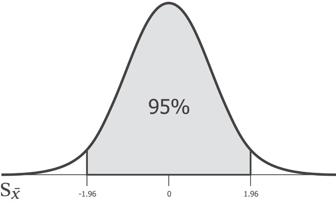
, 95% -1.96 1.96 . , , 1.96 95%- . z-.
z- , z-. , z- — .
1.96 , . , , scipy stats.norm.ppf
. confidence_interval
p 0 1. 95%- 0.95. 2 (2.5% 95%):
def confidence_interval(p, xs):
    ''' '''
    mu = xs.mean()
    se = standard_error(xs)
    z_crit = stats.norm.ppf(1 - (1-p) / 2)
    return [mu - z_crit * se, mu + z_crit * se]

def ex_2_9():
    '''
           '''
    may_1 = '2015-05-01'
    df    = with_parsed_date( load_data('dwell-times.tsv') )
    filtered = df.set_index( ['date'] )[may_1]
    ci = confidence_interval(0.95, filtered['dwell-time'])
    print(' : ', ci)
: [83.53415272762004, 97.753065317492741]
, 95% , 83.53 97.75 . , , , .
- AcmeContent - . , -. .
, , , , :
def ex_2_10():
    '''  ,
          '''
    ts = load_data('campaign-sample.tsv')['dwell-time']
    print('n:                      ', ts.count())
    print(':                ', ts.mean())
    print(':                ', ts.median())
    print(' : ', ts.std())
    print(' :     ', standard_error(ts))

ex_2_10()
n:                       300
:                 130.22
:                 84.0
 :  136.13370714388034
 :      7.846572839994115
, , — 130 . 90 . , , 2 , , . , 95%- , confidence_interval, :
def ex_2_11():
    '''   ,
           '''
    ts = load_data('campaign-sample.tsv')['dwell-time']
    print(' :', confidence_interval(0.95, ts))
: [114.84099983154137, 145.59900016845864]
95%- 114.8 145.6 . 90 . , - , . , .
, , , .
, , . , , , ( ) .
, « » (Literary Digest) 1936 . - : 2.4 . . — - . . 57% . , 62% .
. « » , . , , , , . — , . , .
, - . , . « » , , .
campaign_sample.tsv, , 6 2015 . , pandas:
''' '''
d = pd.to_datetime('2015 6 6')
d.weekday() in [5,6]
True
, . , , , — — , .
— :
def ex_2_12():
    '''
         ,  '''
    df = load_data('dwell-times.tsv')
    means = mean_dwell_times_by_date(df)['dwell-time']
    means.hist(bins=20)
    plt.xlabel('   , .')
    plt.ylabel('')
    plt.show()
:
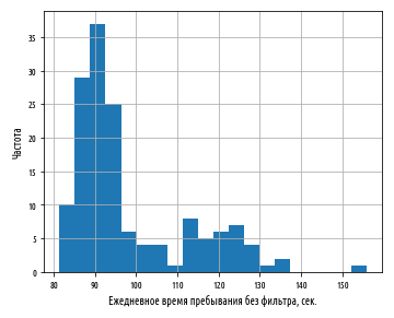
. , . , , .
. , , , , . , , .
. , . :
def ex_2_13():
    '''  ,
           '''
    df = with_parsed_date( load_data('dwell-times.tsv') )
    df.index = df['date']
    df = df[df['date'].index.dayofweek > 4]   # -
    weekend_times = df['dwell-time']

    print('n:                      ', weekend_times.count())
    print(':                ', weekend_times.mean())
    print(':                ', weekend_times.median())
    print(' : ', weekend_times.std())
    print(' :     ', standard_error(weekend_times))
n:                       5860
:                 117.78686006825939
:                 81.0
 :  120.65234077179436
 :      1.5759770362547678
( 6- ) 117.8 . 95%- . , 130 . , , .
( - ), . , . , .
, №3.
Github. .