Python and statistical inference: part 1

“I don’t see anything in her,” I said, returning the hat to Sherlock Holmes.

“No, Watson, you see, but you don’t take the trouble to reflect on what you see.

Arthur Conan Doyle. Blue carbuncle

In the previous series for beginners (first post here ) from a remix of Henry Garner's book Clojure for Data Science in Python, several numerical and visual approaches were presented to understand what a normal distribution is. We discussed several descriptive statistics such as mean and standard deviation, and how they can be used to summarize large amounts of data in a nutshell.

A dataset is usually a sample of a larger population, or general population. Sometimes this population is too large to be fully measured. Sometimes it is immeasurable in nature because it is infinite in size or because it cannot be directly accessed. In any case, we are forced to draw conclusions based on the data at our disposal.

In this 4-post series, we'll look at the statistical implication of how you can go beyond simply describing samples and instead describe the population from which they were drawn. We will take a closer look at our degree of confidence in the inferences we draw from the sampled data. We will reveal the essence of a robust approach to solving problems in the field of data science, which is the testing of statistical hypotheses, which just brings scientificity to the study of data.

In addition, in the course of the presentation, pain points associated with the terminological drift in domestic statistics, sometimes obscuring the meaning and substituting concepts, will be highlighted. At the end of the final post, you can vote for or against the next series of posts. In the meantime ...

, AcmeContent, .

AcmeContent

, , , AcmeContent . -, .

, AcmeContent - — . , -. , , - , - , AcmeContent , .

^{(dwell time)— , - , .}

^{(bounce) — , — .}

, , - - - - - - AcmeContent.

, : scipy, pandas matplotlib. pandas Excel, read_excel



. . pandas read_csv



, URL- .

- AcmeContent — - . :

^{ex_N_M, ex - example (), N - M - . . , .. - . , .}

def load_data( fname ):
    return pd.read_csv('data/ch02/' + fname, '\t')

def ex_2_1():
    return load_data('dwell-times.tsv').head()
      
      

        
        
        
      

    
        
        
        
      
      

        
        
        
      

    
    

( Python Jupyter), , :

, .

, dwell-time hist:

def ex_2_2():
    load_data('dwell-times.tsv')['dwell-time'].hist(bins=50)
    plt.xlabel(' , .')
    plt.ylabel('')
    plt.show()   
      
      

        
        
        
      

    
        
        
        
      
      

        
        
        
      

    
    

:

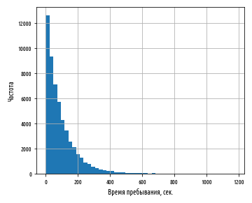
, ; . ( - 0 .). X , , .

, , , Y . , , . , « », . , , .

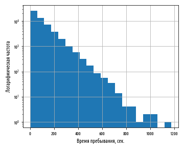
, , . , 10, , 5 10 4 . , — 30 10 20 . — .

Y logy=True



pandas plot.hist



:

def ex_2_3():
    load_data('dwell-times.tsv')['dwell-time'].plot.hist(bins=20, logy=True)
    plt.xlabel(' , .')
    plt.ylabel(' ')
    plt.show()  
      
      

        
        
        
      

    
        
        
        
      
      

        
        
        
      

    
    

pandas , 10 . , , -. , - ( , loglog=True



).

, — . , 10, , , .

— .

( ) , . , , , .

, — . , , . , — , -.

. :

def ex_2_4():
    ts = load_data('dwell-times.tsv')['dwell-time']
    print(':               ', ts.mean())    
    print(':               ', ts.median())
    print(' :', ts.std())
      
      

        
        
        
      

    
        
        
        
      
      

        
        
        
      

    
    

:                 93.2014074074074
:                 64.0
 :  93.96972402519819
      
      

        
        
        
      

    
        
        
        
      
      

        
        
        
      

    
    

. , . — .

^.

( ). . , -, , , -, . 93 ., , 93 ., - .

, , - 93 . , , - 93 ., 5 . , .

x .

, . , ( ).

64 ., - . 93 . , . 6 . , . .

- . , , . Python, pandas — to_datetime.

, date-time, , , 1- Series



pandas , . , errors='ignore'



, . , mean_dwell_times_by_date



resample



. -, . 'D'



, mean



. , dt.resample('D').mean()



:

def with_parsed_date(df):
    '''  date   date-time'''
    df['date'] = pd.to_datetime(df['date'], errors='ignore')
    return df

def filter_weekdays(df): 
    '''   '''
    return df[df['date'].index.dayofweek < 5]  # ..

def mean_dwell_times_by_date(df):
    '''  '''
    df.index = with_parsed_date(df)['date']
    return df.resample('D').mean()  #   

def daily_mean_dwell_times(df):
    '''     -    '''
    df.index = with_parsed_date(df)['date']
    df = filter_weekdays(df)
    return df.resample('D').mean()
      
      

        
        
        
      

    
        
        
        
      
      

        
        
        
      

    
    

, :

def ex_2_5():
    df  = load_data('dwell-times.tsv')    
    mus = daily_mean_dwell_times(df)
    print(':                ', float(means.mean()))    
    print(':                ', float(means.median()))
    print(' : ', float(means.std()))
      
      

        
        
        
      

    
        
        
        
      
      

        
        
        
      

    
    

:                 90.21042865056198
:                 90.13661202185793
 :  3.7223429053200348
      
      

        
        
        
      

    
        
        
        
      
      

        
        
        
      

    
    

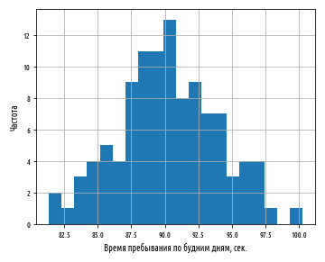
90.2 . , , . , 3.7 . , , . :

def ex_2_6():
    df = load_data('dwell-times.tsv')
    daily_mean_dwell_times(df)['dwell-time'].hist(bins=20)
    plt.xlabel('    , .')
    plt.ylabel('')
    plt.show()
      
      

        
        
        
      

    
        
        
        
      
      

        
        
        
      

    
    

:

, 90 . 3.7 . , , .. , .

, . , , .

^{, , .}

, - , — , , , . , , .

. , , . ( dropna, , ):

def ex_2_7():
    '''    '''
    df = load_data('dwell-times.tsv')
    means = daily_mean_dwell_times(df)['dwell-time'].dropna() 
    ax = means.hist(bins=20, normed=True)
    xs = sorted(means)    # 
    df = pd.DataFrame()
    df[0] = xs
    df[1] = stats.norm.pdf(xs, means.mean(), means.std())
    df.plot(0, 1, linewidth=2, color='r', legend=None, ax=ax)
    plt.xlabel('    , .')
    plt.ylabel('')    
    plt.show()
      
      

        
        
        
      

    
        
        
        
      
      

        
        
        
      

    
    

:

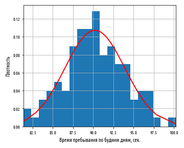
, , , 3.7 . , , 90 . , . 3.7 . — , , .

, (Standard Error, . SE) , , .

^{— .}

, 6 . , , :

σ_x — , x, n — . , . . , — , :

def variance(xs):
    '''  ()  n <= 30'''
    x_hat = xs.mean() 
    n = len(xs)
    n = n-1 if n in range(1, 30) else n  
    square_deviation = lambda x : (x – x_hat) ** 2 
    return sum( map(square_deviation, xs) ) / n

def standard_deviation(xs):
    return sp.sqrt(variance(xs))

def standard_error(xs):
    return standard_deviation(xs) / sp.sqrt(len(xs))
      
      

        
        
        
      

    
        
        
        
      
      

        
        
        
      

    
    

:

• 
  
  
  
  

• 
  
  
  
  

. , , , .

, , , . , .

   Github.    .

The topic of the next post, post # 2 , will be the difference between samples and the population, as well as the confidence interval. Yes, it is the confidence interval , not the confidence interval.