Post # 2 for beginners is about descriptive statistics, data grouping, and normal distribution. All this information will lay the foundation for further analysis of electoral data.
Descriptive statistics
Descriptive statistics, or statistics, are numbers that are used to summarize and describe data. For the purpose of demonstrating what we mean, let's look at the Electorate column. It shows the total number of registered voters in each constituency:
def ex_1_6():
    '''    ""'''
    return load_uk_scrubbed()['Electorate'].count()
650
We have already cleared the column by filtering out empty values ( nan
) from the dataset, and therefore the previous example should return the total number of constituencies.
Descriptive statistics, called summary statistics , are different approaches to measuring the properties of sequences of numbers. They help to characterize the sequence and can act as a guideline for further analysis. Let's start with the two most basic statistics that we can calculate from a sequence of numbers - its mean and variance.
Mean
The most common way to average a dataset is to take the average. The average is actually one of several ways to measure the center of the data distribution . The average value of a numeric series is calculated in Python as follows:
def mean(xs):
    '''   '''
    return sum(xs) / len(xs)
mean
:
def ex_1_7():
    '''    ""'''
    return mean( load_uk_scrubbed()['Electorate'] )
70149.94
, pandas mean, . :
load_uk_scrubbed()['Electorate'].mean()
— . , — , . , , .
def median(xs):
    '''  '''
    n = len(xs)
    mid = n // 2
    if n % 2 == 1:
        return sorted(xs)[mid]
    else:
        return mean( sorted(xs)[mid-1:][:2] )
:
def ex_1_8():
    '''   ""'''
    return median( load_uk_scrubbed()['Electorate'] )
70813.5
pandas , median
.
, . , , 50, , .
, , 5048, 50.
«» . , , , . :

s2 — , .

, square_deviation
, xs
. mean, .
def variance(xs):
    '''  ,
          n <= 30'''
    mu = mean(xs)
    n = len(xs)
    n = n-1 if n in range(1, 30) else n
    square_deviation = lambda x : (x - mu) ** 2
    return sum( map(square_deviation, xs) ) / n
Python **
.
, .. , , .. « ». . , «», . , :
def standard_deviation(xs):
    '''   '''
    return sp.sqrt( variance(xs) )

def ex_1_9():
    '''   ""'''
    return standard_deviation( load_uk_scrubbed()['Electorate'] )
7672.77
pandas , var
std
. , , , ddof=0
, , :
load_uk_scrubbed()['Electorate'].std( ddof=0 )
, .. , . 0 1, 0.5 .
:
[10 11 15 21 22.5 28 30]
, 21 . 0.5-. , 0.0 (), 0.25, 0.5, 0.75 1.0 . , . .
. pandas quantile
. .
def ex_1_10():
    ''' :
           xs,
        p- '''
    q = [0, 1/4, 1/2, 3/4, 1]
    return load_uk_scrubbed()['Electorate'].quantile(q=q)
0.00     21780.00
0.25     65929.25
0.50     70813.50
0.75     74948.50
1.00    109922.00
Name: Electorate, dtype: float64
, , . (0.25) (0.75) , . , .
, , (binning). , Counter
( , ) , . , - , (bins).
, . . , , :

15 x, 5 . , , , , — . Python nbin
:
def nbin(n, xs):
    '''    '''
    min_x, max_x = min(xs), max(xs)
    range_x = max_x - min_x
    fn = lambda x: min( int((abs(x) - min_x) / range_x * n), n-1 )
    return map(fn, xs)
, 0-14 5 :
list( nbin(5, range(15)) )
[0, 0, 0, 1, 1, 1, 2, 2, 2, 3, 3, 3, 4, 4, 4]
, , Counter
, . :
def ex_1_11():
    '''m    5 '''
    series = load_uk_scrubbed()['Electorate']
    return Counter( nbin(5, series) )
Counter({2: 450, 3: 171, 1: 26, 0: 2, 4: 1})
(0 4) , — , , , . .
— . , , , , . , .
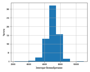
, , pandas hist
, .
def ex_1_12():
    '''
        '''
    load_uk_scrubbed()['Electorate'].hist()
    plt.xlabel(' ')
    plt.ylabel('')
    plt.show()
:
, , , bins
:
def ex_1_13():
    '''
          200 '''
    load_uk_scrubbed()['Electorate'].hist(bins=200)
    plt.xlabel(' ')
    plt.ylabel('')
    plt.show()
, . , , :
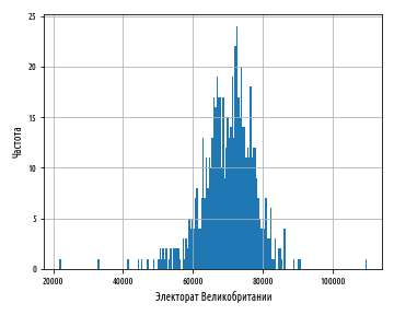
— , , .
def ex_1_14():
    '''
          20 '''
    load_uk_scrubbed()['Electorate'].hist(bins=20)
    plt.xlabel(' ')
    plt.ylabel('')
    plt.show()
20 :

, 20 , , .
, . . — , . , ; , . , , .
, , . .
, , , . , , , .
- , . , , , . , .
: . , . .
. , , , , .
. , scipy stats.uniform.rvs
: . , 0 1 .
def ex_1_15():
    '''
         '''
    xs = stats.uniform.rvs(0, 1, 10000)
    pd.Series(xs).hist(bins=20)
    plt.xlabel(' ')
    plt.ylabel('')
    plt.show()
, Series
pandas .
:
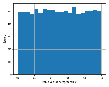
, , . , , . , , , , , . .
, , .
def bootstrap(xs, n, replace=True):
    '''
        n  '''
    return np.random.choice(xs, (len(xs), n), replace=replace)

def ex_1_16():
    '''   '''
    xs = stats.uniform.rvs(loc=0, scale=1, size=10000)
    pd.Series( map(sp.mean, bootstrap(xs, 10)) ).hist(bins=20)
    plt.xlabel('  ')
    plt.ylabel('')
    plt.show()
, :
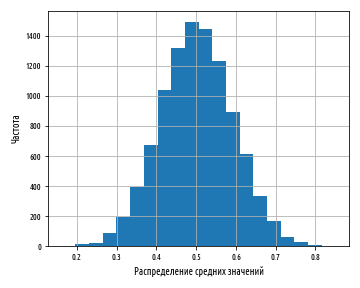
0 1 , . , .
, , , , , .
20- , 1733 . M, , . . , , scipy , :
def ex_1_17():
    '''
         '''
    xs = stats.norm.rvs(loc=0, scale=1, size=10000)
    pd.Series(xs).hist(bins=20)
    plt.xlabel(' ')
    plt.ylabel('')
    plt.show()
, sp.random.normal
loc
– , scale
– size
– . :

By default, the mean and standard deviation for a normal distribution are 0 and 1, respectively.
The source code examples for this post are in my Github repo . All source data is taken from the repo of the author of the book.
The next part, part 3 , of the "Python, Data Science and Choices" post series is devoted to generating distributions, their properties, and graphs for their comparative analysis.