Dates and times are not easy objects:
- months contain a different number of days;
- years are leap years and not;
- there are different time zones;
- hours, minutes, days use different number systems;
- and many other nuances.
The following is a summary of some points that are rarely highlighted in the documentation, as well as tricks that allow you to write fast and controlled code.
A very short summary for smartphone readers: on large amounts of data, we use only POSIXct
fractional seconds. It will be good, of course, quickly.
It is a continuation of a series of previous publications .
Standards for Specifying Dates and Times
ISO 8601 Data elements and interchange formats - Information interchange - Representation of dates and times is an international standard covering the exchange of date- and time-related data.
Basic R Methods for Working with Time
date
Sys.Date()
print("-----")
x <- as.Date("2019-01-29") # UTC
print(x)
tz(x)
str(x)
dput(x)
print("-----")
dput(as.Date("1970-01-01")) # ! origin
## [1] "2021-04-29" ## [1] "-----" ## [1] "2019-01-29" ## [1] "UTC" ## Date[1:1], format: "2019-01-29" ## structure(17925, class = "Date") ## [1] "-----" ## structure(0, class = "Date")
Non-standard date format during initialization must be specified specially
as.Date("04/20/2011", format = "%m/%d/%Y")
## [1] "2011-04-20"
Time
There are two basic types of time used in R: POSIXct
and POSIXlt
.
The external views POSIXct
and POSIXlt
look similar. And the internal ones?
z <- Sys.time()
glue(" ",
"POSIXct - {z}",
"POSIXlt - {as.POSIXlt(z)}", "---", .sep = "\n")
glue(" ",
"POSIXct - {capture.output(dput(z))}",
"POSIXlt - {paste0(capture.output(dput(as.POSIXlt(z))), collapse = '')}",
"---", .sep = "\n")
# /
glue(": {year(z)} \n: {minute(z)}\n: {second(z)}\n---")
## ## POSIXct - 2021-04-29 15:18:04 ## POSIXlt - 2021-04-29 15:18:04 ## --- ## ## POSIXct - structure(1619698684.50764, class = c("POSIXct", "POSIXt")) ## POSIXlt - structure(list(sec = 4.50764489173889, min = 18L, hour = 15L, mday = 29L, mon = 3L, year = 121L, wday = 4L, yday = 118L, isdst = 0L, zone = "MSK", gmtoff = 10800L), class = c("POSIXlt", "POSIXt"), tzone = c("", "MSK", "MSD")) ## --- ## : 2021 ## : 18 ## : 4 ## ---
We immediately conclude that for serious work with data (more than 10 lines with time), we POSIXlt
forget about it as a bad dream. It's a complex structure with insane overhead.
POSIXct
unixtimestamp, () ( 0 01.01.1970). .
— online unixtimestamp:
- Epoch Unix Time Stamp Converter
- Epoch & Unix Timestamp Conversion Tools
- currentDate / Time in Millisecondsmillis
z <- 1548802400
as.POSIXct(z, origin = "1970-01-01") # local
as.POSIXct(z, origin = "1970-01-01", tz = "UTC") # in UTC
## [1] "2019-01-30 01:53:20 MSK" ## [1] "2019-01-29 22:53:20 UTC"
. . :
- ISO, (ISO 8601-2019);
- - ;
- .
POSIXct
, - . :
x <- ymd_hms("2014-09-24 15:23:10")
x
x + 0.5
x + 0.5 + 0.6
options(digits.secs=5)
x + 0.45756
options(digits.secs=0)
x
## [1] "2014-09-24 15:23:10 UTC" ## [1] "2014-09-24 15:23:10 UTC" ## [1] "2014-09-24 15:23:11 UTC" ## [1] "2014-09-24 15:23:10.45756 UTC" ## [1] "2014-09-24 15:23:10 UTC"
, .
options(digits.secs=5)
# generate data
df <- data.frame(
timestamp = as_datetime(
round(runif(20, min = now() - seconds(10), max = now()), 0),
tz ="Europe/Moscow")) %>%
mutate(ms = round(runif(n(), 0, 999), 0)) %>%
mutate(value = round(runif(n(), 0, 100), 0))
dput(df)
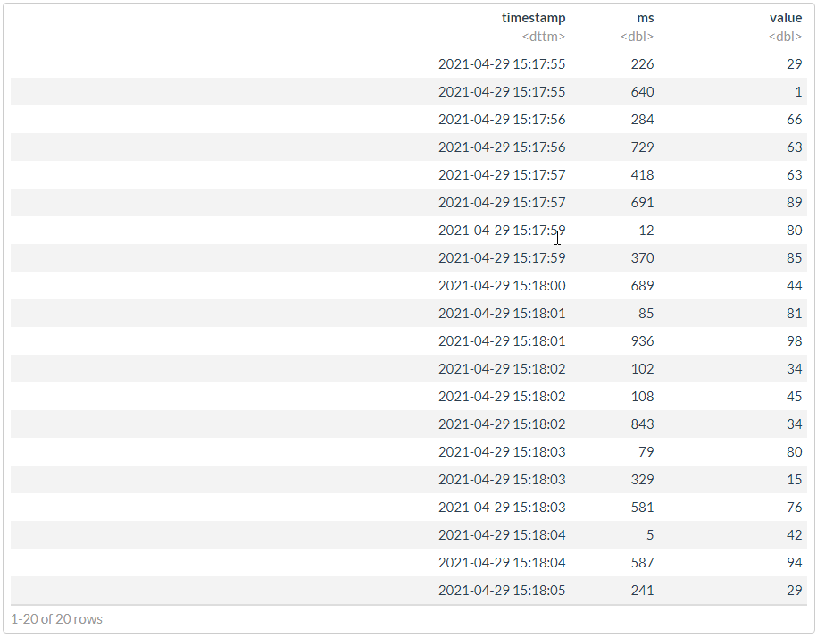
# " "
df %>%
arrange(timestamp, ms)
options(digits.secs=0)
## structure(list(timestamp = structure(c(1619698677, 1619698680, ## 1619698676, 1619698682, 1619698675, 1619698682, 1619698679, 1619698679, ## 1619698684, 1619698683, 1619698684, 1619698677, 1619698682, 1619698683, ## 1619698675, 1619698676, 1619698685, 1619698681, 1619698683, 1619698681 ## ), class = c("POSIXct", "POSIXt"), tzone = "Europe/Moscow"), ## ms = c(418, 689, 729, 108, 226, 843, 12, 370, 5, 581, 587, ## 691, 102, 79, 640, 284, 241, 85, 329, 936), value = c(63, ## 44, 63, 45, 29, 34, 80, 85, 42, 76, 94, 89, 34, 80, 1, 66, ## 29, 81, 15, 98)), class = "data.frame", row.names = c(NA, ## -20L))
# ""
# [magrittr aliases](https://magrittr.tidyverse.org/reference/aliases.html)
df2 <- df %>%
mutate(timestamp = timestamp + ms/1000) %>%
# mutate_at("timestamp", ~`+`(. + ms/1000)) %>%
select(-ms) %>%
df2 %>% arrange(timestamp)

#
dt <- as.data.table(df2)
bench::mark(
naive = dplyr::arrange(df, timestamp, ms),
smart = dplyr::arrange(df2, timestamp),
dt = dt[order(timestamp)],
check = FALSE,
relative = TRUE,
min_iterations = 1000
)
## # A tibble: 3 x 6 ## expression min median `itr/sec` mem_alloc `gc/sec` ## <bch:expr> <dbl> <dbl> <dbl> <dbl> <dbl> ## 1 naive 11.9 11.8 1 1.06 1 ## 2 smart 11.1 11.0 1.06 1 1.06 ## 3 dt 1 1 11.6 494. 1.22
.
data <- c("05102019210003657", "05102019210003757", "05102019210003857")
dmy_hms(stri_c(stri_sub(data, to = 14L), ".", stri_sub(data, from = 15L)), tz = "Europe/Moscow")
#
data2 <- data %>%
sample(10^6, replace = TRUE)
bench::mark(
stri_sub = stri_c(stri_sub(data2, to = 14L), ".", stri_sub(data2, from = 15L)),
stri_replace = stri_replace_first_regex(data2, pattern = "(^.{14})(.*)", replacement = "$1.$2"),
re2_replace = re2_replace(data2, pattern = "(^.{14})(.*)", replacement = "\\1.\\2", parallel = TRUE)
)
## [1] "2019-10-05 21:00:03 MSK" "2019-10-05 21:00:03 MSK" ## [3] "2019-10-05 21:00:03 MSK" ## # A tibble: 3 x 6 ## expression min median `itr/sec` mem_alloc `gc/sec` ## <bch:expr> <bch:tm> <bch:tm> <dbl> <bch:byt> <dbl> ## 1 stri_sub 214ms 222ms 4.10 22.89MB 5.47 ## 2 stri_replace 653ms 653ms 1.53 7.63MB 0 ## 3 re2_replace 409ms 413ms 2.42 15.29MB 1.21
lubridate
x <- ymd(20101215)
print(x)
class(x)
## [1] "2010-12-15" ## [1] "Date"
lubridate
ymd(20101215) == mdy("12/15/10")
## [1] TRUE
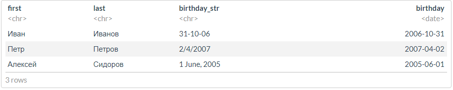
df <- tibble(first = c("", "", ""),
last = c("", "", ""),
birthday_str = c("31-10-06", "2/4/2007", "1 June, 2005")) %>%
mutate(birthday = dmy(birthday_str))
df
, ?
# lubridate
options(lubridate.verbose = TRUE)
# : ..
df <- tibble(time_str = c("08.05.19 12:04:56", "09.05.19 12:05", "12.05.19 23"))
lubridate::dmy_hms(df$time_str, tz = "Europe/Moscow")
print("---------------------")
lubridate::dmy(df$time_str, tz = "Europe/Moscow")
## [1] "2019-05-08 12:04:56 MSK" NA ## [3] NA ## [1] "---------------------" ## [1] NA NA NA
# lubridate
options(lubridate.verbose = TRUE)
lubridate::dmy_hms(df$time_str, truncated = 3, tz = "Europe/Moscow")
## [1] "2019-05-08 12:04:56 MSK" "2019-05-09 12:05:00 MSK" ## [3] "2019-05-12 23:00:00 MSK"
# lubridate
options(lubridate.verbose = TRUE)
# : ..
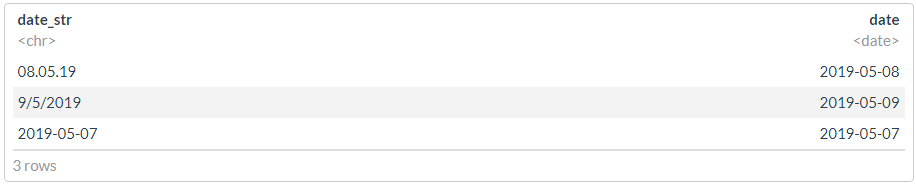
df <- tibble(date_str = c("08.05.19", "9/5/2019", "2019-05-07"))
#
glimpse(dmy(df$date_str))
print("---------------------")
#
glimpse(ymd(df$date_str))
print("---------------------")
## Date[1:3], format: "2019-05-08" "2019-05-09" NA ## [1] "---------------------" ## Date[1:3], format: "2008-05-19" NA "2019-05-07" ## [1] "---------------------"
? , , , - .
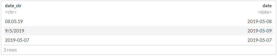
df %>% mutate(date = dplyr::coalesce(dmy(date_str), ymd(date_str)))
df1 <- df
df1$date <- dmy(df1$date_str)
idx <- is.na(df1$date)
print("---------------------")
idx
df1$date[idx] <- ymd(df1$date_str[idx])
print("---------------------")
df1
## [1] "---------------------" ## [1] FALSE FALSE TRUE ## [1] "---------------------"
"" :
POSIXct
options(lubridate.verbose = FALSE)
date1 <- ymd_hms("2011-09-23-03-45-23")
date2 <- ymd_hms("2011-10-03-21-02-19")
# ?
as.numeric(date2) - as.numeric(date1) # ,
(date2 - date1) %>% dput()
difftime(date2, date1)
difftime(date2, date1, unit="mins")
difftime(date2, date1, unit="secs")
## [1] 926216 ## structure(10.7200925925926, class = "difftime", units = "days") ## Time difference of 10.72009 days ## Time difference of 15436.93 mins ## Time difference of 926216 secs
date1 <- ymd_hms("2019-01-30 00:00:00")
date1
date1 - days(1)
date1 + days(1)
date1 + days(2)
## [1] "2019-01-30 UTC" ## [1] "2019-01-29 UTC" ## [1] "2019-01-31 UTC" ## [1] "2019-02-01 UTC"
—
date1 - months(1)
date1 + months(1) # !!!
## [1] "2018-12-30 UTC" ## [1] NA
. , .
date1 %m-% months(1)
date1 %m+% months(1)
date1 %m+% months(1) %m-% months(1)
## [1] "2018-12-30 UTC" ## [1] "2019-02-28 UTC" ## [1] "2019-01-28 UTC"
date1 <- ymd_hms("2019-01-30 01:00:00")
date1 %T>% print() %>% dput()
with_tz(date1, tzone = "Europe/Moscow") %T>% print() %>% dput()
force_tz(date1, tzone = "Europe/Moscow") %T>% print() %>% dput()
## [1] "2019-01-30 01:00:00 UTC" ## structure(1548810000, class = c("POSIXct", "POSIXt"), tzone = "UTC") ## [1] "2019-01-30 04:00:00 MSK" ## structure(1548810000, class = c("POSIXct", "POSIXt"), tzone = "Europe/Moscow") ## [1] "2019-01-30 01:00:00 MSK" ## structure(1548799200, class = c("POSIXct", "POSIXt"), tzone = "Europe/Moscow")
, , ? , hms
. .
hms_str <- "03:22:14"
as_hms(hms_str)
dput(as_hms(hms_str))
print("-------")
x <- as_hms(hms_str) * 15
x
str(x)
# seconds_to_period(period_to_seconds(x))
seconds_to_period(x) %T>% dput() %>% print()
## 03:22:14 ## structure(12134, units = "secs", class = c("hms", "difftime")) ## [1] "-------" ## Time difference of 182010 secs ## 'difftime' num 182010 ## - attr(*, "units")= chr "secs" ## new("Period", .Data = 30, year = 0, month = 0, day = 2, hour = 2, ## minute = 33) ## [1] "2d 2H 33M 30S"
— . .
( Clickhouse) , , unixtimestamp UTC. , .
:
- . timestamp, , , , , .
- ( ). , , , .
- unixtimestamp UTC , . (!).
- , timestamp. ,
X-1
X+1
, .
, 0.
.
(, ) . , :
- , ;
- ;
- ;
- ( );
- ;
-
double
; - ;
- .
-- ClickHouse
SELECT DISTINCT
store, pos,
timestamp, ms,
concat(toString(store), '-', toString(pos)) AS pos_uid,
toFloat64(timestamp) + (ms / 1000) AS timestamp
flog.info(paste("SQL query:", sql_req))
tic(" CH")
raw_df <- dbGetQuery(conn, stri_encode(sql_req, to = "UTF-8")) %>%
mutate_if(is.character, `Encoding<-`, "UTF-8") %>%
as_tibble() %>%
mutate_at(vars(timestamp), anytime::anytime, tz = "Europe/Moscow") %>%
mutate_at("event", as.factor)
flog.info(capture.output(toc()))
DBI::dbDisconnect(conn)
data.frame
#
df -> as_tibble(_df) %>%
map(pryr::object_size) %>%
unlist() %>%
enframe() %>%
arrange(desc(value)) %>%
mutate_at("value", fs::as_fs_bytes) %>%
mutate(ratio = formattable::percent(value / sum(value), 2)) %>%
add_row(name = "TOTAL", value = sum(.$value))
,
- Epoch & Unix Timestamp Conversion Tools
- currentdate/time in millisecondsmillis
- Functions for working with dates and times
, , , . .
df <- seq.Date(from = as.Date("2021-01-01"),
to = as.Date("2021-05-31"),
by = "2 days") %>%
# sample(20, replace = FALSE) %>%
tibble(date = .)
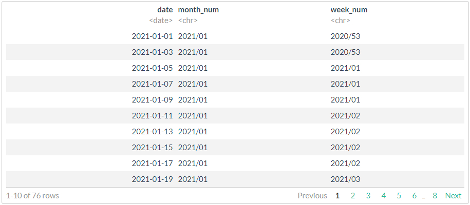
# //
# 1
df %>%
mutate(month_num = stri_c(lubridate::year(date),
sprintf("%02d", lubridate::month(date)),
sep = "/"),
week_num = stri_c(lubridate::isoyear(date),
sprintf("%02d", lubridate::isoweek(date)),
sep = "/")
)
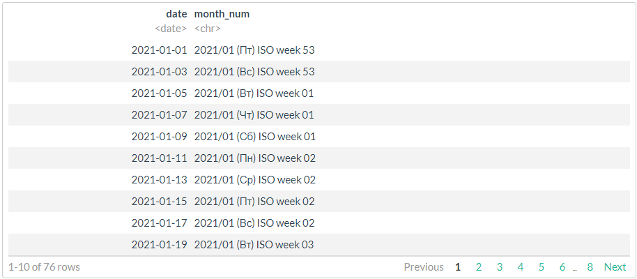
# //
# 2,
# , !!!
df %>%
mutate(month_num = format(date, "%Y/%m (%a) ISO week %V"))
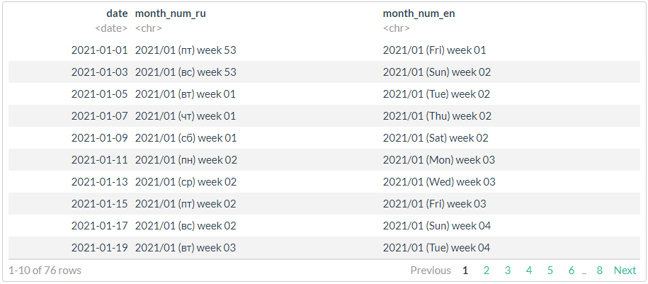
# //
# 3,
# strptime (ISO 8601) ICU
# https://man7.org/linux/man-pages/man3/strptime.3.html
stri_datetime_fstr("%Y/%m (%a) week %V")
# ggthemes::tableau_color_pal("Tableau 20")(20) %>% scales::show_col()
# , !!!
df %>%
mutate(
month_num_ru = stri_datetime_format(
date, "yyyy'/'MM' ('ccc') week 'ww", locale = "ru", tz = "UTC"),
month_num_en = stri_datetime_format(
date, "yyyy'/'MM' ('ccc') week 'ww", locale = "en", tz = "UTC"))
. .
stri_datetime_format(today(), "LLLL", locale="ru@calendar=Persian")
stri_datetime_format(today(), "LLLL", locale="ru@calendar=Indian")
stri_datetime_format(today(), "LLLL", locale="ru@calendar=Hebrew")
stri_datetime_format(today(), "LLLL", locale="ru@calendar=Islamic")
stri_datetime_format(today(), "LLLL", locale="ru@calendar=Coptic")
stri_datetime_format(today(), "LLLL", locale="ru@calendar=Ethiopic")
stri_datetime_format(today(), "dd MMMM yyyy", locale="ru")
stri_datetime_format(today(), "LLLL d, yyyy", locale="ru")
## [1] "" ## [1] "" ## [1] "" ## [1] "" ## [1] "" ## [1] "" ## [1] "29 2021" ## [1] " 29, 2021"
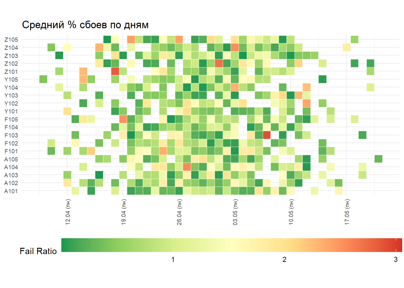
.
#
map_tbl <- tibble(
date = as_date(Sys.time() + rnorm(10^3, mean = 0, sd = 60 * 60 * 24 * 7))) %>%
mutate(store = stri_c(sample(c("A", "F", "Y", "Z"), n(), replace = TRUE),
sample(101:105, n(), replace = TRUE))) %>%
mutate(store_fct = as.factor(store)) %>%
mutate(fail_ratio = abs(rnorm(n(), mean = 0.3, sd = 1)))
my_date_format <- function (format = "dd MMMM yyyy", tz = "Europe/Moscow")
{
scales:::force_all(format, tz)
# stri_datetime_fstr("%d.%m%n%A")
# stri_datetime_fstr("%d.%m (%a)")
function(x) stri_datetime_format(x, format, locale = "ru", tz = tz)
}
# ,
gp <- map_tbl %>%
ggplot(aes(x = date, y = store_fct, fill = fail_ratio)) +
geom_tile(color = "white", size = 0.1) +
# scale_fill_distiller(palette = "RdYlGn", name = "Fail Ratio", label = comma) +
# scale_fill_distiller(palette = "RdYlGn", name = "Fail Ratio", guide = guide_legend(keywidth = unit(4, "cm"))) +
scale_fill_distiller(palette = "RdYlGn", name = "Fail Ratio") +
scale_x_date(breaks = scales::date_breaks("1 week"), labels = my_date_format("dd'.'MM' ('ccc')'")) +
coord_equal() +
labs(x = NULL, y = NULL, title = " % ") +
theme_minimal() +
theme(plot.title = element_text(hjust = 0)) +
theme(axis.ticks = element_blank()) +
theme(axis.text = element_text(size = 7)) +
theme(axis.text.x = element_text(angle = 90, vjust = 0.5)) +
theme(legend.position = "bottom") +
theme(legend.key.width = unit(3, "cm"))
gp
base_df <- tibble(
start = Sys.time() + rnorm(10^3, mean = 0, sd = 60 * 24 * 3)) %>%
mutate(finish = start + rnorm(n(), mean = 100, sd = 60)) %>%
mutate(user_id = sample(as.character(1000:1100), n(), replace = TRUE)) %>%
arrange(user_id, start)
dt <- as.data.table(base_df, key = c("user_id", "start")) %>%
.[, c("start", "finish") := lapply(.SD, as.numeric),
.SDcols = c("start", "finish")]
df <- group_by(base_df, user_id)
bench::mark(
dplyr_v1 = df %>% transmute(delta_t = as.numeric(difftime(finish, start, units = "secs"))) %>% ungroup(),
dplyr_v2 = ungroup(df) %>% transmute(delta_t = as.numeric(difftime(finish, start, units = "secs"))),
dplyr_v3 = dt %>% transmute(delta_t = finish - start),
dt_v1 = dt[, .(delta_t = finish - start), by = user_id],
dt_v2 = dt[, .(delta_t = finish - start)],
check = FALSE # all_equal
)
## # A tibble: 5 x 6 ## expression min median `itr/sec` mem_alloc `gc/sec` ## <bch:expr> <bch:tm> <bch:tm> <dbl> <bch:byt> <dbl> ## 1 dplyr_v1 4.3ms 4.86ms 200. 103.1KB 11.4 ## 2 dplyr_v2 2.17ms 2.46ms 380. 17.9KB 6.24 ## 3 dplyr_v3 1.67ms 1.77ms 527. 29.8KB 8.51 ## 4 dt_v1 410.4us 438.7us 2139. 90.8KB 8.35 ## 5 dt_v2 304.4us 335.3us 2785. 264.6KB 8.38
: //. , , ?
Sample code. Do not forget that a number of functions work taking into account the locale of the machine on which the code is executed. And if your month is printed in Russian, then this does not guarantee (if you do not use methods) similar behavior on another machine or another OS.
# https://stackoverflow.com/questions/16347731/how-to-change-the-locale-of-r
# https://jangorecki.gitlab.io/data.cube/library/stringi/html/stringi-locale.html
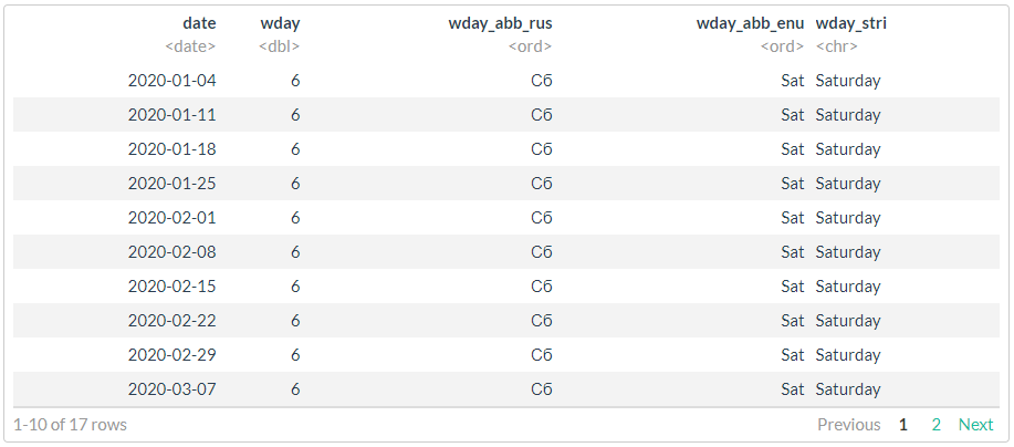
df <- as.Date("2020-01-01") %>%
seq.Date(to = . + months(4), by = "1 day") %>%
tibble(date = .) %>%
mutate(wday = lubridate::wday(date, week_start = 1),
wday_abb_rus = lubridate::wday(date, label = TRUE, week_start = 1),
wday_abb_enu = lubridate::wday(date, label = TRUE, week_start = 1, locale = "English"),
wday_stri = stringi::stri_datetime_format(date, "EEEE", locale = "en"))
#
filter(df, wday == 6)
PS Most of the tests are for example only. You can run it on your machines, the numbers will be completely different, but the nature of the dependence and ratio should be approximately the same.
Previous post - "R vs Python in a productive loop" .