Computer vision is a field of computer science that focuses on reproducing parts of a complex human vision system and allows computers to identify and process objects in images and videos, as well as people. Early experiments in computer vision began in the 1950s and were first commercially used to distinguish between printed and handwritten text in the 1970s. Today, computer vision applications have grown exponentially. This article shows an example of how you can recognize road signs using computer vision.

, Kaggle: GTSRB — , (IJCNN) 2011. 50 000 43 . : , - .
.
import os
import matplotlib
import numpy as np
from PIL import Image
from tensorflow.keras.preprocessing.image import img_to_array
from sklearn.model_selection import train_test_split
from keras.utils import to_categorical
from keras.models import Sequential, load_model
from keras.layers import Conv2D, MaxPool2D, Dense, Flatten, Dropout
from tensorflow.keras import backend as K
import matplotlib.pyplot as plt
from sklearn.metrics import accuracy_score
«train», 43 . : data labels. , , .
data = [] labels = []
, os data labels. PIL.
for num in range(0, classes):
path = os.path.join('train',str(num))
imagePaths = os.listdir(path)
for img in imagePaths:
image = Image.open(path + '/'+ img)
image = image.resize((30,30))
image = img_to_array(image)
data.append(image)
labels.append(num)
30×30 data labels.
numpy .
data = np.array(data) labels = np.array(labels)
- (39209, 30, 30, 3), , 39 209 30×30 , 3 , ( RGB).
print(data.shape, labels.shape)
(39209, 30, 30, 3) (39209,)
sklearn
train_test_split()
, 80% 20% . .
X_train, X_test, y_train, y_test = train_test_split(data, labels, test_size=0.2, random_state=42)
print(X_train.shape, X_test.shape, y_train.shape, y_test.shape)
(31367, 30, 30, 3) (7842, 30, 30, 3) (31367,) (7842,)
, .
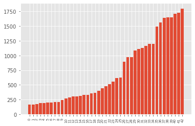
def cnt_img_in_classes(labels):
count = {}
for i in labels:
if i in count:
count[i] += 1
else:
count[i] = 1
return count
samples_distribution = cnt_img_in_classes (y_train)
def diagram(count_classes):
plt.bar(range(len(dct)), sorted(list(count_classes.values())), align='center')
plt.xticks(range(len(dct)), sorted(list(count_classes.keys())), rotation=90, fontsize=7)
plt.show()
diagram(samples_distribution)

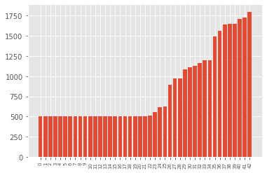
, , , .
def aug_images(images, p):
from imgaug import augmenters as iaa
augs = iaa.SomeOf((2, 4),
[
iaa.Crop(px=(0, 4)),
iaa.Affine(scale={"x": (0.8, 1.2), "y": (0.8, 1.2)}),
iaa.Affine(translate_percent={"x": (-0.2, 0.2), "y": (-0.2, 0.2)}),
iaa.Affine(rotate=(-45, 45))
iaa.Affine(shear=(-10, 10))
])
seq = iaa.Sequential([iaa.Sometimes(p, augs)])
res = seq.augment_images(images)
return res
def augmentation(images, labels):
min_imgs = 500
classes = cnt_img_in_classes(labels)
for i in range(len(classes)):
if (classes[i] < min_imgs):
add_num = min_imgs - classes[i]
imgs_for_augm = []
lbls_for_augm = []
for j in range(add_num):
im_index = random.choice(np.where(labels == i)[0])
imgs_for_augm.append(images[im_index])
lbls_for_augm.append(labels[im_index])
augmented_class = augment_imgs(imgs_for_augm, 1)
augmented_class_np = np.array(augmented_class)
augmented_lbls_np = np.array(lbls_for_augm)
imgs = np.concatenate((images, augmented_class_np), axis=0)
lbls = np.concatenate((labels, augmented_lbls_np), axis=0)
return (images, labels)
X_train, y_train = augmentation(X_train, y_train)
.
print(X_train.shape, X_test.shape, y_train.shape, y_test.shape)
(36256, 30, 30, 3) (7842, 30, 30, 3) (36256,) (7842,)
.
augmented_samples_distribution = cnt_img_in_classes(y_train) diagram(augmented_samples_distribution)

, . keras.utils
to_categorical
, y_train
t_test
, one-hot encoding.
y_train = to_categorical(y_train, 43)
y_test = to_categorical(y_test, 43)
Keras]. , CNN ( ). CNN .
:
2 Conv2D (filter=32, kernel_size=(5,5), activation=”relu”)
MaxPool2D ( pool_size=(2,2))
Dropout (rate=0.25)
2 Conv2D (filter=64, kernel_size=(3,3), activation=”relu”)
MaxPool2D ( pool_size=(2,2))
Dropout (rate=0.25)
Flatten , 1
Dense (500, activation=”relu”)
Dropout (rate=0.5)
Dense (43, activation=”softmax”)
class Net:
@staticmethod
def build(width, height, depth, classes):
model = Sequential()
inputShape = (height, width, depth)
if K.image_data_format() == 'channels_first':
inputShape = (depth, heigth, width)
model = Sequential()
model.add(Conv2D(filters=32, kernel_size=(5,5), activation='relu', input_shape=inputShape))
model.add(Conv2D(filters=32, kernel_size=(5,5), activation='relu'))
model.add(MaxPool2D(pool_size=(2, 2)))
model.add(Dropout(rate=0.25))
model.add(Conv2D(filters=64, kernel_size=(3, 3), activation='relu'))
model.add(Conv2D(filters=64, kernel_size=(3, 3), activation='relu'))
model.add(MaxPool2D(pool_size=(2, 2)))
model.add(Dropout(rate=0.25))
model.add(Flatten())
model.add(Dense(500, activation='relu'))
model.add(Dropout(rate=0.5))
model.add(Dense(classes, activation='softmax'))
return model
Adam
, — categorical_crossentropy
, . model.fit()
.
epochs = 25
model = Net.build(width=30, height=30, depth=3, classes=43)
model.compile(loss='categorical_crossentropy', optimizer='adam', metrics=['accuracy'])
history = model.fit(X_train, y_train, batch_size=64, validation_data=(X_test, y_test), epochs=epochs)

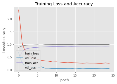
, 25 93% . matplotlib
.
plt.style.use("plot")
plt.figure()
N = epochs
plt.plot(np.arange(0, N), history.history["loss"], label="train_loss")
plt.plot(np.arange(0, N), history.history["val_loss"], label="val_loss")
plt.plot(np.arange(0, N), history.history["accuracy"], label="train_acc")
plt.plot(np.arange(0, N), history.history["val_accuracy"], label="val_acc")
plt.title("Training Loss and Accuracy")
plt.xlabel("Epoch")
plt.ylabel("Loss/Accuracy")
plt.legend(loc="lower left")
plt.show()

The dataset contains a "Test" folder, and the file Test.csv
contains information associated with the image path and class labels. We extract the path to the image and labels from the file Test.csv
using the framework Pandas
. Then, we resize the image to 30x30 pixels and make an array numpy
containing all of the image data. Using accuracy_score
from, we sklearn metrics
check the accuracy of the predictions of our model. We have achieved 96% accuracy on this model.
y_test = pd.read_csv('Test.csv')
labels = y_test["ClassId"].values
imgs = y_test["Path"].values
images=[]
for img in imgs:
image = Image.open(img)
image = image.resize((30,30))
images.append(img_to_array(image))
X_test=np.array(images)
pred = model.predict_classes(X_test)
print(accuracy_score(labels, pred))
0.958590657165479