
Hello, Habr!
In this article, we will look at a few simple time series forecasting approaches.
The material presented in the article, in my opinion, well complements the first week of the course "Applied Problems of Data Analysis" from MIPT and Yandex. On the indicated course, you can get theoretical knowledge sufficient to solve the problems of predicting the series of dynamics, and as a practical consolidation of the material, it is proposed using the ARIMA model of the scipy library to generate a salary forecast in the Russian Federation for the year ahead. In the article, we will also generate a salary forecast, but at the same time we will use not the scipy library , but the library sklearn . The trick is that scipy already has an ARIMA model , but sklearn does not have a ready-made model, so we have to work hard with pens. Thus, in order to solve the problem, in a sense, we will need to figure out how the model works from the inside. Also, as additional material, in the article, the prediction problem is solved using a single-layer neural network of the pytorch library .
All code is written in python 3 in jupyter notebook . Moreover, the notebook is designed in such a way that instead of data on wages, you can substitute many other series of dynamics, for example, data on sugar prices, change the forecasting, validation and training period, add other external factors and form an appropriate forecast. In other words, a simple self-written simulator is used in the work, with the help of which it is possible to predict various series of dynamics. The code can be viewed here
Article outline
- Brief description of the simulator.
- A head-on solution is to forecast time series using only "raw" data of past values of time series.
- Adding exogenous variables.
- Correction of heteroscedasticity through the logarithm of the initial data.
- Bringing the row to a stationary one.
- Forecasting with a single layer neural network.
- Comparison of approaches.
- useful links
Brief description of the simulator
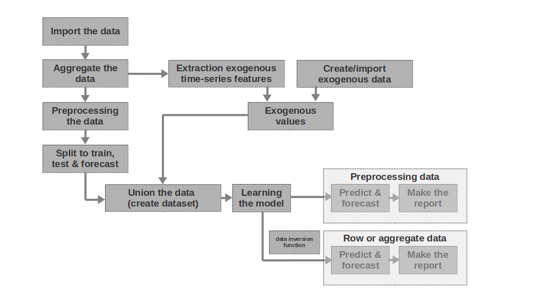
Import the data
Everything is simple here - we import the data. Sometimes it happens that raw data is enough to form a more or less intelligible forecast. It is the first and second forecasts in the article that are modeled on the basis of raw data, that is, raw data on wages in past periods are used to forecast wages.
Aggregate the data
The article does not use data aggregation because it is not necessary. However, data can often be presented at unequal time intervals. In this case, you just need to aggregate them. For example, data from trading in securities, currencies and other financial instruments must be aggregated. Usually, the average value in the interval is taken, but the maximum, minimum, standard deviation and other statistics are also possible.
Preprocessing the data
In our case, we are talking primarily about data preprocessing, due to which the time series acquires the property of homoscedasticity (through the logarithm of the data) and becomes stationary (through the differentiation of the series).
Split to train, test & forecast
In this block of code, the time series is divided into periods of training, testing and forecasting by adding a new column with the corresponding values "train", "test", "forecast". That is, we do not create three separate tables for each period, but simply add a column, based on which we will further divide the data.
Extraction exogenous time-series features
It can be useful to isolate additional external (exogenous) features from a time series. For example, indicate whether it is a day off or not, indicate the number of days in a month (or the number of working days in a month), etc. As a rule, these signs are "pulled out" from the time series itself without any manual intervention.
Create / import exogenous data
Not all information can be “pulled” from the time series. Sometimes additional external data may be required. For example, some episodic events that have a strong impact on the values of the time series. Such events can be the dates of the beginning of hostilities, the imposition of sanctions, natural disasters, etc. The work does not consider such factors, but the possibility of their use should be borne in mind.
Exogenous values
In this block of code, we combine all exogenous data into one table.
Union the data (create dataset)
In this block of code, we combine the values of the time series and exogenous features into one table. In other words, we are preparing a dataset, on the basis of which we will train the model, test the quality and form a forecast.
Learning the model
Everything is clear here - we are just training the model.
Preprocessing data: predict & forecast
If we used pre-processed data for training the model (logarithmic, processed by the box-coke function, stationary series, etc.), then the quality of the model is first evaluated on the preprocessed data and only then on the "raw" data. If we did not preprocess the data, then this stage is skipped.
Row data: predict & forecast
This stage is the final one. If the model was trained on pre-processed data, for example, we prologized them, then to get the forecast of wages in rubles, and not the logarithm of rubles, we should translate the forecast back into rubles.
I would also like to note that the article uses a one-dimensional time series to predict wages. However, nothing prevents you from using a multidimensional series, for example, adding data on the exchange rate of the ruble to the dollar or some other series.
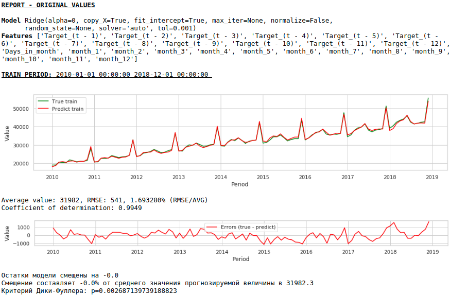
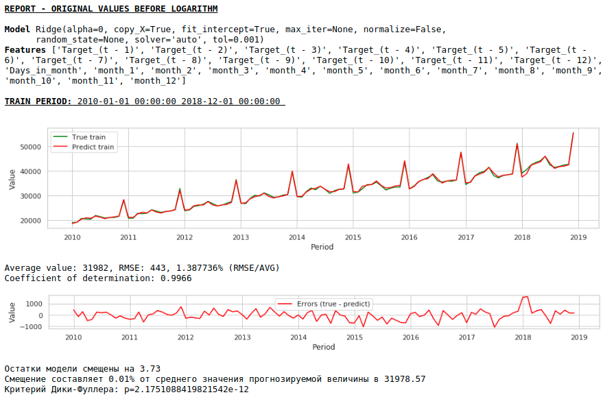
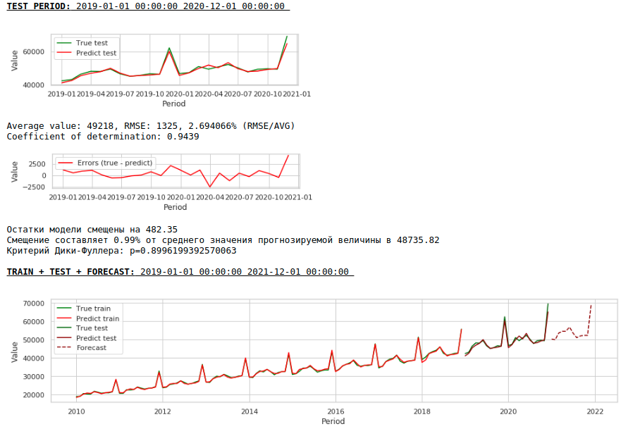
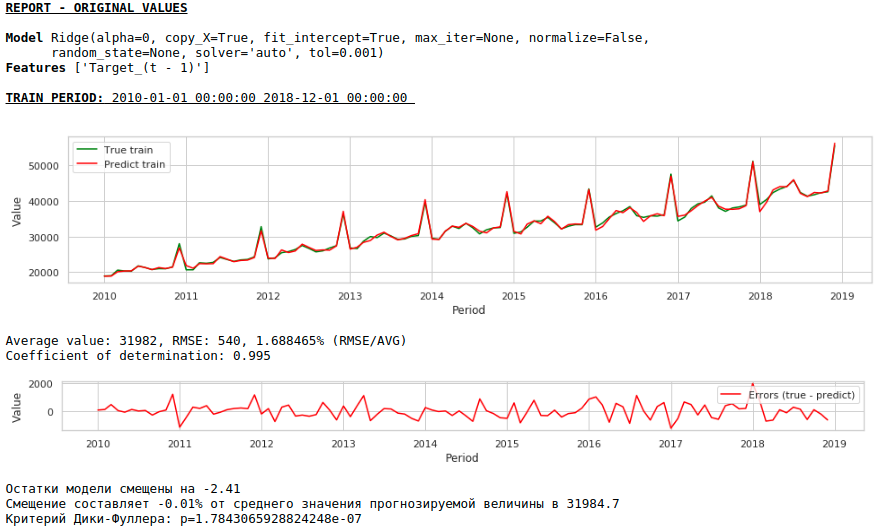
Decision in the forehead
We will assume that data on wages in the past can approximate wages in the future. In other words, the size of wages, for example, in January depends on what wages were in December, November, October, ...
Let's take the values of wages in the past 12 months to predict wages in the 13th month. In other words, for each target value, we will have 12 features.
The signs will be fed to the Ridge Regression input of the sklearn library. We take the default parameters of the model, except for the alpha parameter, it was set to 0, that is, in fact, we are using regular regression.
This is a straightforward solution - it is the simplest :) There are situations when you need to give at least some result very urgently, but there is simply no time for any preprocessing or there is not enough experience to quickly process or add data. In such situations, you can use raw data as a baseline to build a forecast. Looking ahead, I note that the quality of the model turned out to be comparable to the quality of models that use data preprocessing.
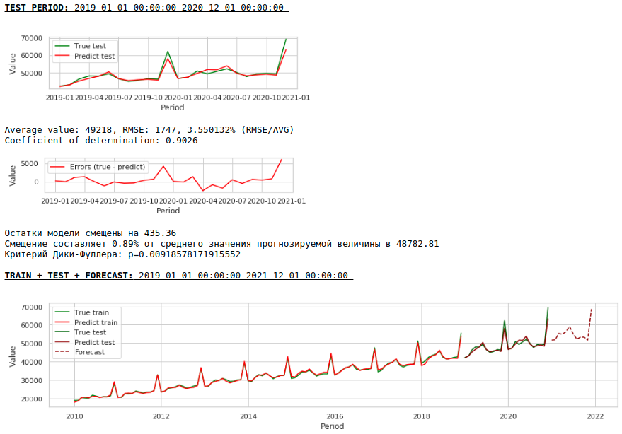
Let's see what we got.
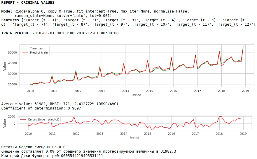
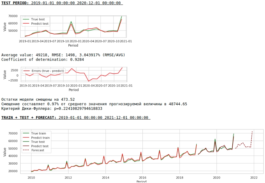
At first glance, the result looks, though imperfect, but close to reality.
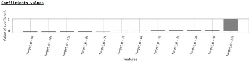
In accordance with the values of the regression coefficients, the value of the salary has the greatest influence on the forecast of wages exactly a year ago.
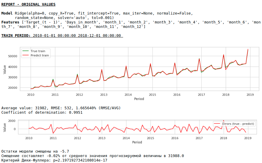
Let's try to add exogenous variables to the model.
Adding exogenous variables
We will use 2 external signs: the number of days in a month and the number of the month (from 1 to 12). We binarize the attribute "Month number", as a result we get 12 columns for each month with values of 0 or 1.
Let's form a new dataset and look at the quality of the model.
Watching charts
The quality is lower. Visually, it is noticeable that the forecast does not look entirely plausible in terms of wage growth in December.
Let's now do the first data preprocessing.
Correction of heteroscedasticity.
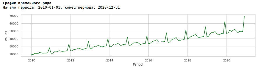
If we look at the wage chart for the period from 2010 to 2020, we will see that the spread of wages within the year between months is growing every year.
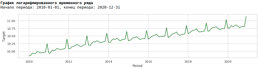
An annual increase in variance from month to month leads to heteroscedasticity. To improve the quality of forecasting, we should get rid of this property of the data and bring them to homoscedasticity.
To do this, we will use the usual logarithm and see how the logarithmic series looks like.
Let's train the model on the logarithmic series
Watching charts
As a result, the quality of predictions on the training and test samples did improve, however, the forecast for 2021 visually looks less plausible compared to the forecast of the first model. Most likely, the use of exogenous factors degrades the model.
Bringing a row to a stationary
We will reduce the series to a stationary one as follows:
- Determine the difference between the target salary value and the value a year ago: t - (t-12) = dif_1
- Determine the difference between the received and shifted by 1 month value: dif_1 - (dif_1-1) = dif_2
As a result, we get the following time series.
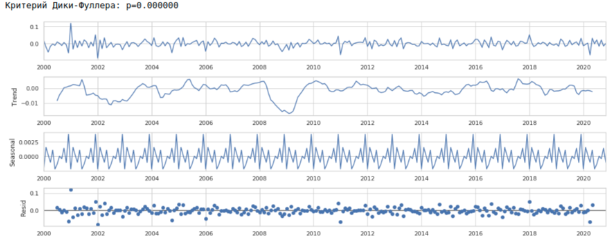
The series really looks stationary, this is also indicated by the value of the Dickey-Fuller criterion.
It is not necessary to expect a good quality of predictions on the training and test samples on the processed data, that is, on a stationary series, since in fact, in this case, the model should predict the values of white noise. But for us, to predict wages, it is not at all necessary to use regression, since, by reducing the series to a stationary one, we, in simple terms, have determined a formula for approximating the target variable. But we will not deviate from the canons and will use a regression model, besides, we have exogenous factors.
Let's see what happened.
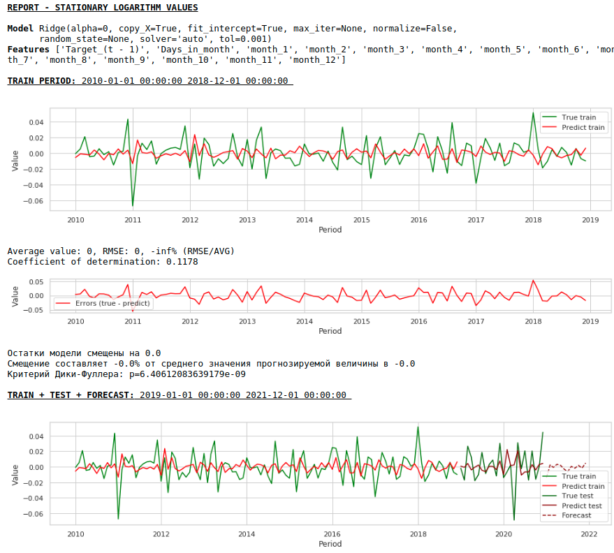
This is how the prediction of a stationary series looks like. As expected - not very good :)
And here is the prediction and forecast of wages.
Watching charts
The quality has improved markedly and the forecast is visually believable.
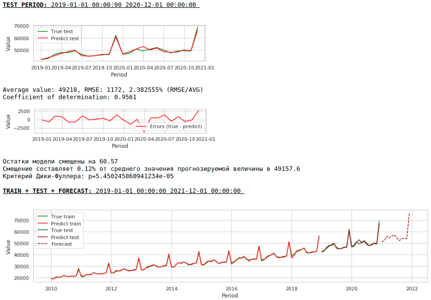
Now let's make a forecast without using exogenous variables.
Watching charts

The quality has improved further and the plausibility of the forecast is preserved :)
Forecasting with a single layer neural network
We will feed the existing datasets to the input of the neural network. Since our network is single-layer, in fact this is the same linear regression with simple modifications and you should not expect a very large difference in the quality of predictions.
First, let's take a look at the network itself.
See the code
class Model_1(nn.Module):
    def __init__(self, input_size, output_size):
        super(Model_1, self).__init__()
        self.input_size = input_size
        self.output_size = output_size
        self.linear = nn.Linear(self.input_size, self.output_size)

    def forward(self, x):
        output = self.linear(x)
        return output
Now a few words about how we will train her.
- We fix a random seed for the purpose of reproducibility of the result
- Initializing the model
- Setting the loss function - MSELoss
- Selecting Adam optimizer as the optimizer
- We indicate the initial step of training and determine the condition under which the step is lowered. Note that the correct choice of a step and its further change (usually a decrease) brings good results.
- Specify the number of learning epochs
- We start training
- We supply the entire dataset to the network input, since it is very small and it makes no sense to break it into batches
- During training, every thousand epochs we form graphs of the value of the loss function on the training and test samples. This allows us to control overfitting or not retraining the model.
Below is the code for training the network on the first dataset. For each dataset, the parameters changed slightly: the number of training epochs and the training step.
See the code
# fix the random seed
SEED = 42
random_init(SEED)

# initialization model, loss function, optimizator
model = Model_1(len(features),1)
loss_func = nn.MSELoss()
opt = torch.optim.Adam(model.parameters(), lr=5e-2)

# set the epoch numbers, initialization list for every loss after learning on epoch
epochs = 15000
losses_train = []
losses_test = []
# initialization counter for calculation epoch numbers
counter = 0
# start the learning model
for epoch in range(epochs):
    model.train()
#     make prediction targets on train data
    y_pred_train = model(torch.tensor(X_train.to_numpy(), dtype=torch.float))
#     calculate loss
    loss = loss_func(y_pred_train,
                     torch.reshape(torch.tensor(y_train.to_numpy(), dtype=torch.float),(-1,1)))
#     bacward loss to model and calculate new parameters (coefficients) with fixed learning rate
    loss.backward()
    opt.step()
    opt.zero_grad()

# add loss to list losses
    losses_train.append(loss)

    model.eval()
    y_pred_test = model(torch.tensor(X_test.to_numpy(), dtype=torch.float))
    loss_test = loss_func(y_pred_test,
                     torch.reshape(torch.tensor(y_test.to_numpy(), dtype=torch.float),(-1,1)))
    losses_test.append(loss_test)


# make the mini report for every 1000 epoch
    if epoch % 1000 == 0 and epoch > 0:
        print ('Epoch:', epoch // 1000)
        print ('Learning rate:', opt.param_groups[0]['lr'])
        print ('Last loss on TRAIN data:', losses_train[-1].cpu().detach().numpy(),
              '              Last loss on TEST data:', losses_test[-1].cpu().detach().numpy())
#         print ('Last loss on TEST data:', losses_test[-1].cpu().detach().numpy())
        fig, (ax1, ax2) = plt.subplots(1, 2)
#         fig.suptitle('MSE on TRAIN & TEST DATA')
        fig.set_figheight(3)
        fig.set_figwidth(12)
        ax1.plot(np.arange(counter,epoch,1), np.array([float(i) for i in losses_train][-1000:]), color = 'darkred')
        plt.xlabel("Epoch")
        plt.ylabel("Loss on TRAIN data")
        ax2.plot(np.arange(counter,epoch,1), np.array([float(i) for i in losses_test][-1000:]), color = 'darkred')
        plt.xlabel("Epoch")
        plt.ylabel("Loss on TEST data")
        plt.show()

        counter += 1000

#   reduce learning rate
    if epoch == 1000:
        opt = torch.optim.Adam(model.parameters(), lr=7e-3)
We will not consider the quality of predictions for each dataset separately (those who wish can see the details on the gita). Let's compare the final results.
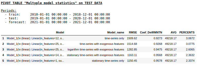
Quality on a test sample using Ridge Regression
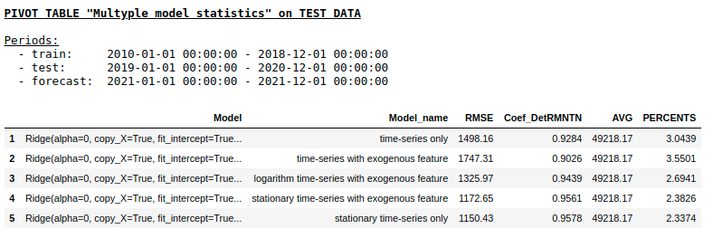
Quality on a test sample using Single layer NN
As we expected, there was no fundamental difference between regular regression and a simple single layer neural network. Of course, neurons provide more maneuver for learning: you can change optimizers, adjust learning steps, use hidden layers and activation functions, you can go even further and use recurrent neural networks - RNNs. By the way, personally, I was not able to get sane quality in this problem using RNN, however, on the Internet, you can find many interesting examples of time series forecasting using LSTM.
At this point, the article came to an end. I hope the material will be useful as a kind of overview of baseline approaches used in forecasting time series and will serve as a good practical addition to the course "Applied Problems of Data Analysis" from MIPT and Yandex.
useful links
- Sources on github
- Course "Applied Data Analysis Problems" from MIPT and Yandex
- State statistics "EMISS" (data on wages)
- LSTM for time series prediction
- Lecture 9. Forecasting based on a regression model. Computer Science Center
- The picture under the title is taken from here :)