🙅🏿 👨🏽‍🎓 👩🏻‍🏭 Feature selection in machine learning problems. Part 1 🚅 🦖 👨🏾‍💻

Often, the datasets that you have to work with contain a large number of features, the number of which can reach several hundred or even thousands. When building a machine learning model, it is not always clear which of the features are really important for it (i.e. have a connection with the target variable), and which are redundant (or noise). Removing redundant features allows you to better understand the data, as well as reduce the time of model tuning, improve its accuracy and facilitate interpretability. Sometimes this task can even be the most significant, for example, finding the optimal set of features can help to decipher the mechanisms underlying the problem under study. This can be useful for the development of various methodologies such as bank scoring, fraud detection or medical diagnostic tests.Feature selection methods are generally divided into 3 categories: filter methods, embedded methods, and wrapper methods. The choice of the appropriate method is not always obvious and depends on the task and the available data. The purpose of this series of articles is to provide a brief overview of some of the popular feature selection methods, with a discussion of their merits, demerits, and implementation features. The first part is about filters and built-in methods.The first part is about filters and built-in methods.The first part is about filters and built-in methods.

1. Filtration methods

Filtering techniques are applied prior to model training and generally have low computational costs. These include visual analysis (for example, removal of a feature that has only one value, or most of the values are missing), assessment of features using some statistical criterion (variance, correlation, X ² , etc.) and expert judgment (removal of features that do not fit in their meaning, or signs with incorrect values).

The simplest way to assess the suitability of features is by exploratory data analysis (for example, with the pandas-profiling library ). This task can be automated using the feature-selector library , which selects features based on the following parameters:

( ).
( , ).
( , ).
lightgbm ( , lightgbm. lightgbm .)

sklearn. VarianceThreshold , . SelectKBest SelectPercentile , . F-,

F-

F- , . sklearn f_regression f_classif .

X²

. ( sklearn). , .

( ). - " " . sklearn mutual_info_regression mutual_info_classif .

2.

, . ( L1) ( ). , .

– , $50 . , :

age –
fnlwgt (final weight) – ,
educational-num –
capital-gain –
capital-loss –
hours-per-week –

import pandas as pd
import numpy as np
import matplotlib.pyplot as plt
import seaborn as sns
from sklearn.feature_selection import GenericUnivariateSelect, mutual_info_classif, SelectFromModel
from sklearn.pipeline import Pipeline
from sklearn.model_selection import StratifiedKFold, GridSearchCV, cross_val_score
from sklearn.ensemble import RandomForestClassifier
from sklearn.preprocessing import PowerTransformer
from sklearn.linear_model import LogisticRegression

#        
SEED = 1

# ,    
def plot_features_scores(model, data, target, column_names, model_type):
    '''    '''
    
    model.fit(data, target)
    
    if model_type == 'rf':
        (pd.DataFrame(data={'score': model['rf'].feature_importances_}, 
                      index=column_names).sort_values(by='score')
                                         .plot(kind='barh', grid=True,
                                               figsize=(6,6), legend=False));
    elif model_type == 'lr':
        (pd.DataFrame(data={'score': model['lr'].coef_[0]},
                      index=column_names).sort_values(by='score')
                                         .plot(kind='barh', grid=True,
                                               figsize=(6,6), legend=False));
        
    else:
        raise KeyError('Unknown model_type')

def grid_search(model, gs_params):
    '''       '''
     
    gs = GridSearchCV(estimator=model, param_grid=gs_params, refit=True,
                      scoring='roc_auc', n_jobs=-1, cv=skf, verbose=0)
    gs.fit(X, y)
    scores = [gs.cv_results_[f'split{i}_test_score'][gs.best_index_] for i in range(5)]
    print('scores = {}, \nmean score = {:.5f} +/- {:.5f} \
           \nbest params = {}'.format(scores,
                                      gs.cv_results_['mean_test_score'][gs.best_index_],
                                      gs.cv_results_['std_test_score'][gs.best_index_],
                                      gs.best_params_))
    return gs
        
#          
df = pd.read_csv(r'..\adult.data.csv')

# ,    
#    
X = df.select_dtypes(exclude=['object']).copy()
#   
y = df['salary'].map({'<=50K':0, '>50K':1}).values

X.head()

	age	fnlwgt	education-num	capital-gain	hours-per-week
0	39	77516	13	2174	40
1	50	83311	13	0	13
2	38	215646	9	0	40
3	53	234721	7	0	40
4	28	338409	13	0	40

X.describe()

	age	fnlwgt	education-num	capital-gain	capital-loss	hours-per-week
count	32561.000000	3.256100e+04	32561.000000	32561.000000	32561.000000	32561.000000
mean	38.581647	1.897784e+05	10.080679	1077.648844	87.303830	40.437456
std	13.640433	1.055500e+05	2.572720	7385.292085	402.960219	12.347429
min	17.000000	1.228500e+04	1.000000	0.000000	0.000000	1.000000
25%	28.000000	1.178270e+05	9.000000	0.000000	0.000000	40.000000
50%	37.000000	1.783560e+05	10.000000	0.000000	0.000000	40.000000
75%	48.000000	2.370510e+05	12.000000	0.000000	0.000000	45.000000
max	90.000000	1.484705e+06	16.000000	99999.000000	4356.000000	99.000000

- :

rf = Pipeline([('rf', RandomForestClassifier(n_jobs=-1, 
                                             class_weight='balanced', 
                                             random_state=SEED))])

#  - ( 5-  ) 
skf = StratifiedKFold(n_splits=5, shuffle=True, random_state=SEED)

scores = cross_val_score(estimator=rf, X=X, y=y, 
                         cv=skf, scoring='roc_auc', n_jobs=-1)
print('scores = {} \nmean score = {:.5f} +/- {:.5f}'.format(scores, scores.mean(), scores.std()))

#  
plot_features_scores(model=rf, data=X, target=y, column_names=X.columns, model_type='rf')

scores = [0.82427915 0.82290796 0.83106668 0.8192637  0.83155106] 
mean score = 0.82581 +/- 0.00478

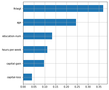
fnlwgt. , , $50 . . , , ( ). , , , .

( L1-). PowerTransformer.

lr = Pipeline([('p_trans', PowerTransformer(method='yeo-johnson', standardize=True)),
               ('lr', LogisticRegression(solver='liblinear',
                                         penalty='l1',
                                         max_iter=200,
                                         class_weight='balanced',
                                         random_state=SEED)
               )])
scores = cross_val_score(estimator=lr, X=X, y=y, 
                         cv=skf, scoring='roc_auc', n_jobs=-1)
print('scores = {} \nmean score = {:.5f} +/- {:.5f}'.format(scores, scores.mean(), scores.std()))

plot_features_scores(model=lr, data=X, target=y, column_names=X.columns, model_type='lr')

scores = [0.82034993 0.83000963 0.8348707  0.81787667 0.83548066] 
mean score = 0.82772 +/- 0.00732

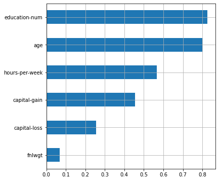
12 , , . .

#       
np.random.seed(SEED)

fix, (ax1, ax2, ax3) = plt.subplots(nrows=1, ncols=3, figsize=(14,5))
ax1.set_title("normal distribution")
ax2.set_title("uniform distribution")
ax3.set_title("laplace distribution")
for i in range(4):
    X.loc[:, f'norm_{i}'] = np.random.normal(loc=np.random.randint(low=0, high=10), 
                                             scale=np.random.randint(low=1, high=10), 
                                             size=(X.shape[0], 1))
    
    X.loc[:, f'unif_{i}'] = np.random.uniform(low=np.random.randint(low=1, high=4), 
                                              high=np.random.randint(low=5, high=10), 
                                              size=(X.shape[0], 1))
    X.loc[:, f'lapl_{i}'] = np.random.laplace(loc=np.random.randint(low=0, high=10), 
                                              scale=np.random.randint(low=1, high=10), 
                                              size=(X.shape[0], 1))
    #   
    sns.kdeplot(X[f'norm_{i}'], ax=ax1)
    sns.kdeplot(X[f'unif_{i}'], ax=ax2)
    sns.kdeplot(X[f'lapl_{i}'], ax=ax3)

#  
X.head()

	age	fnlwgt	education-num	capital-gain	hours-per-week	norm_0	unif_0	lapl_0	norm_1	unif_1	lapl_1	norm_2	unif_2	lapl_2	norm_3	unif_3	lapl_3
0	39	77516	13	2174	40	0.246454	4.996750	2.311467	6.474587	6.431455	-0.932124	3.773136	3.382773	-1.324387	8.031167	2.142457	8.050902
1	50	83311	13	0	13	-4.656718	4.693542	2.095298	14.622329	2.795007	6.465348	-3.275117	3.787041	0.652694	7.537461	5.247103	9.014559
2	38	215646	9	0	40	12.788669	4.255611	22.278713	9.643720	3.533265	2.716441	4.725608	3.126107	23.410698	1.932907	4.933431	13.233319
3	53	234721	7	0	40	-15.713848	3.989797	5.971506	8.978198	7.772238	-5.402306	5.742672	3.084132	0.937932	9.435720	4.915537	-3.396526
4	28	338409	13	0	40	20.703306	3.159246	8.718559	8.217148	4.365603	14.403088	3.023828	6.934299	4.978327	7.355296	2.551361	10.479218

- :

scores = cross_val_score(estimator=rf, X=X, y=y, 
                         cv=skf, scoring='roc_auc', n_jobs=-1)
print('scores = {} \nmean score = {:.5f} +/- {:.5f}'.format(scores, scores.mean(), scores.std()))
plot_features_scores(model=rf, data=X, target=y, column_names=X.columns, model_type='rf')

scores = [0.8522425  0.85382173 0.86249657 0.84897581 0.85443027] 
mean score = 0.85439 +/- 0.00447

, - , ! , , . , , , ( – , ) . , .

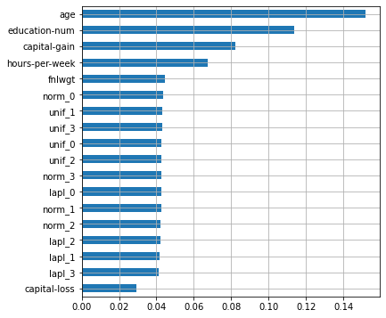
scores = cross_val_score(estimator=lr, X=X, y=y, 
                         cv=skf, scoring='roc_auc', n_jobs=-1)
print('scores = {} \nmean score = {:.5f} +/- {:.5f}'.format(scores, scores.mean(), scores.std()))

plot_features_scores(model=lr, data=X, target=y, column_names=X.columns, model_type='lr')

scores = [0.81993058 0.83005516 0.83446553 0.81763029 0.83543145] 
mean score = 0.82750 +/- 0.00738

, , . , .

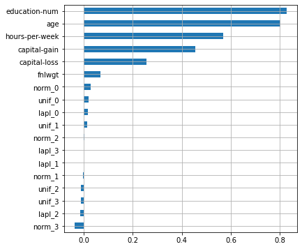
, SelectKBest

SelectPercentile

, GenericUnivariateSelect. 3 – , . .

selector = GenericUnivariateSelect(score_func=mutual_info_classif, 
                                   mode='k_best', 
                                   param=6)
#    
selector.fit(X, y)
#  transform     
#      
pd.DataFrame(data={'score':selector.scores_,
                   'support':selector.get_support()}, 
             index=X.columns).sort_values(by='score',ascending=False)

	score	support
capital-gain	0.080221	True
age	0.065703	True
education-num	0.064743	True
hours-per-week	0.043655	True
capital-loss	0.033617	True
fnlwgt	0.033390	True
norm_3	0.003217	False
unif_3	0.002696	False
norm_0	0.002506	False
norm_2	0.002052	False
lapl_3	0.001201	False
unif_1	0.001144	False
lapl_1	0.000000	False
unif_2	0.000000	False
lapl_2	0.000000	False
lapl_0	0.000000	False
unif_0	0.000000	False
norm_1	0.000000	False

(scores_

), (get_support()=False

).

( ) GenericUnivariateSelect

- . , , :

#       
selector = ('selector', GenericUnivariateSelect(score_func=mutual_info_classif, 
                                                mode='k_best'))
rf.steps.insert(0, selector)

    
# grid search
rf_params = {'selector__param': np.arange(4,10),
             'rf__max_depth': np.arange(2, 16, 2),
             'rf__max_features': np.arange(0.3, 0.9, 0.2)}
print('grid search results for rf')
rf_grid = grid_search(model=rf, gs_params=rf_params)

grid search results for rf
scores = [0.8632776968200635, 0.8683443340928604, 0.8710308000627435, 0.8615748939138762, 0.8693334091828478], 
mean score = 0.86671 +/- 0.00364            
best params = {'rf__max_depth': 12, 'rf__max_features': 0.3, 'selector__param': 5}

- , 5 :

#  ,  
selected_features = [X.columns[i] for i, support
                     in enumerate(rf_grid.best_estimator_['selector'].get_support()) if support]

plot_features_scores(model=rf_grid.best_estimator_, 
                     data=X, target=y, column_names=selected_features, model_type='rf')

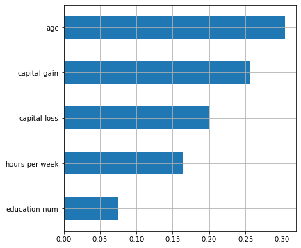
fnlwgt, . GenericUnivariateSelect

. – , . , .

, .

lr_params = {'lr__C': np.logspace(-3, 1.5, 10)}
             
print('grid search results for lr')
lr_grid = grid_search(model=lr, gs_params=lr_params)

plot_features_scores(model=lr_grid.best_estimator_, 
                     data=X, target=y, column_names=X.columns, model_type='lr')

grid search results for lr
scores = [0.820445329307105, 0.829874053687009, 0.8346493482101578, 0.8177211039148669, 0.8354590546776963], 
mean score = 0.82763 +/- 0.00729            
best params = {'lr__C': 0.01}

- , . , (L1) .

. SelectFromModel, .

lr_selector = SelectFromModel(estimator=lr_grid.best_estimator_['lr'], prefit=True, threshold=0.1)

#    
pd.DataFrame(data={'score':lr_selector.estimator.coef_[0],
                   'support':lr_selector.get_support()}, 
             index=X.columns).sort_values(by='score',ascending=False)

	score	support
education-num	0.796547	True
age	0.759419	True
hours-per-week	0.534709	True
capital-gain	0.435187	True
capital-loss	0.237207	True
fnlwgt	0.046698	False
norm_0	0.010349	False
unif_0	0.002101	False
norm_2	0.000000	False
unif_3	0.000000	False
lapl_2	0.000000	False
unif_2	0.000000	False
norm_1	0.000000	False
lapl_1	0.000000	False
unif_1	0.000000	False
lapl_0	0.000000	False
lapl_3	0.000000	False
norm_3	-0.018818	False

. ( ) . – , , , , . , , ( , , , ).

Built-in methods, unlike filters, require more computational resources, as well as more precise configuration and data preparation. However, these methods can reveal more complex dependencies. For a less biased interpretation of the feature coefficients, it is necessary to adjust the regularization of the model. It is important to remember that the distribution of coefficients for linear models depends on the method of data preprocessing.

The methods of feature selection described in the article can be combined, or their hyperparameters can be compared and fitted using the means of sklearn or special libraries .

Feature selection in machine learning problems. Part 1

1. Filtration methods

F-

2.

More articles: