
This article discusses the Home Credit Default Risk machine learning competition , which aims to use historical data on loan applications to predict whether an applicant will be able to repay a loan (determine the risk of a borrower's default). Predicting whether a customer will repay a loan or run into trouble is a critical business challenge, and Home Credit is running a competition on the Kaggle platform to see what machine learning models the community can develop to help them with this challenge.
This is a standard supervised classification task:
Supervised Learning: Correct answers are included in the training data, and the goal is to train the model to predict these responses based on the available cues.
: , – 0 ( ) 1 ( ).
Home Credit, () , . 7 :
applicationtrain / applicationtest: Home Credit. , SKIDCURR . TARGET :
0, ;
1, .
bureau: . , .
bureaubalance: . . , .
previousapplication: Home Credit , . , SKIDPREV.
POSCASHBALANCE: , Home Credit. , .
creditcardbalance: , Home Credit. . .
installments_payment: Home Credit, .
, :

, ( HomeCredit_columns_description.csv) .
(application_train / application_test), . , . , ! - , .
: ROC AUC
( ), , . , (ROC AUC, AUROC).
ROC AUC , , .
(ROC) , , , , :
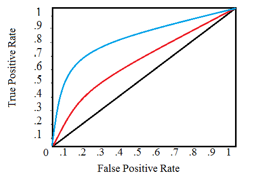
, , . 0 1 . , , . , , , , , , ( ).
(AUC) . ROC ( ). 0 1, . , , ROC AUC = 0,5.
ROC AUC, 0 1, 0 1. , , , ( , ) — . , , 99,9999%, , , . , ( ), , ROC AUC F1, . ROC AUC , ROC AUC .
, , . , , . .
: numpy pandas , sklearn preprocessing , matplotlib ¨C11C¨C12C¨C13C . .
import os
import numpy as np
import pandas as pd
pd.set_option('display.max_columns', None)
from sklearn.preprocessing import LabelEncoder
import matplotlib.pyplot as plt
import seaborn as sns
#
import warnings
warnings.filterwarnings('ignore')
, , . 9 : ( ), ( ), 6 , .
#
print(os.listdir("../input/"))
‘POSCASHbalance.csv’, ‘bureaubalance.csv’, ‘applicationtrain.csv’, ‘previousapplication.csv’, ‘installmentspayments.csv’, ‘creditcardbalance.csv’, ‘samplesubmission.csv’, ‘applicationtest.csv’, ‘bureau.csv’]
#
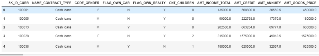
app_train = pd.read_csv('../input/application_train.csv')
print('Training data shape: ', app_train.shape)
app_train.head()
Training data shape: (307511, 122)

307511 , 120 , , .
#
app_test = pd.read_csv('../input/application_test.csv')
print('Testing data shape: ', app_test.shape)
app_test.head()
Testing data shape: (48744, 121)
, TARGET.
(EXPLORATORY DATA ANALYSIS – EDA)
(EDA) — , , , , . EDA — , . , , . , , , , .
— , : 0, , 1, . , .
app_train['TARGET'].value_counts()

app_train['TARGET'].astype(int).plot.hist();
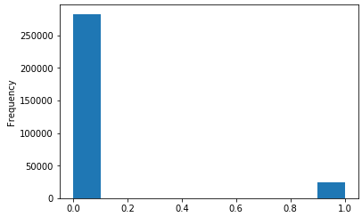
.
#
def missing_values_table(df):
#
mis_val = df.isnull().sum()
#
mis_val_percent = 100 * df.isnull().sum() / len(df)
#
mis_val_table = pd.concat([mis_val, mis_val_percent], axis=1)
#
mis_val_table_ren_columns = mis_val_table.rename(
columns = {0 : 'Missing Values', 1 : '% of Total Values'})
#
mis_val_table_ren_columns = mis_val_table_ren_columns[
mis_val_table_ren_columns.iloc[:,1] != 0].sort_values(
'% of Total Values', ascending=False).round(1)
#
print("Your selected dataframe has " + str(df.shape[1]) + " columns.\n"
"There are " + str(mis_val_table_ren_columns.shape[0]) +
" columns that have missing values.")
return mis_val_table_ren_columns
#
missing_values = missing_values_table(app_train)
missing_values.head(10)
Your selected dataframe has 122 columns.
There are 67 columns that have missing values.

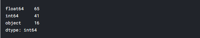
. int64 float64 — ( ). object .
#
app_train.dtypes.value_counts()
object().
#
app_train.select_dtypes('object').apply(pd.Series.nunique, axis = 0)

, . .
, . , ( , LightGBM). , () , . :
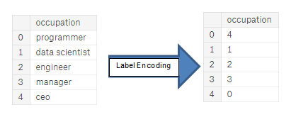
(Label encoding): . . :
(One-hot encoding): . 1 0 .

, . , , - . 4, — 1, , . . , , (, = 4 = 1) , , . (, / ), , .
, , . – Kaggle-master Will Koehrsen, , , . . , ( ) - . , PCA , ( , ).
Label Encoding 2 One-Hot Encoding 2 . , , , , . - .
Label Encoding One-Hot Encoding
: (dtype == object) , – .
LabelEncoder Scikit-Learn, – pandas get_dummies(df).
# label encoder
le = LabelEncoder()
le_count = 0
#
for col in app_train:
if app_train[col].dtype == 'object':
# 2
if len(list(app_train[col].unique())) <= 2:
# LabelEncoder
le.fit(app_train[col])
#
app_train[col] = le.transform(app_train[col])
app_test[col] = le.transform(app_test[col])
# , LabelEncoder
le_count += 1
print('%d columns were label encoded.' % le_count)
3 columns were label encoded.
# one-hot encoding
app_train = pd.get_dummies(app_train)
app_test = pd.get_dummies(app_test)
print('Training Features shape: ', app_train.shape)
print('Testing Features shape: ', app_test.shape)
raining Features shape: (307511, 243)
Testing Features shape: (48744, 239).
(). , , . . ( , ). , axis = 1, , !
train_labels = app_train['TARGET']
# , ,
app_train, app_test = app_train.align(app_test, join = 'inner', axis = 1)
#
app_train['TARGET'] = train_labels
print('Training Features shape: ', app_train.shape)
print('Testing Features shape: ', app_test.shape)
Training Features shape: (307511, 240)
Testing Features shape: (48744, 239)
, . «» . - , , ( , ), .
, EDA, — . - , , . describe. DAYS_BIRTH , . , -1 :
(app_train['DAYS_BIRTH'] / -365).describe()

— . .
app_train['DAYS_EMPLOYED'].describe()
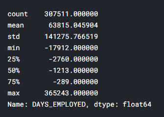
– ( , ) — 1000 !
app_train['DAYS_EMPLOYED'].plot.hist(title = 'Days Employment Histogram');
plt.xlabel('Days Employment');
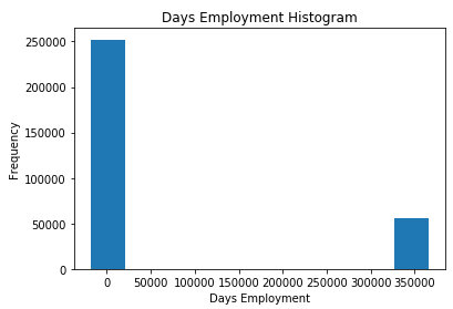
, .
anom = app_train[app_train['DAYS_EMPLOYED'] == 365243]
non_anom = app_train[app_train['DAYS_EMPLOYED'] != 365243]
print('The non-anomalies default on %0.2f%% of loans' % (100 * non_anom['TARGET'].mean()))
print('The anomalies default on %0.2f%% of loans' % (100 * anom['TARGET'].mean()))
print('There are %d anomalous days of employment' % len(anom))
The non-anomalies default on 8.66% of loans
The anomalies default on 5.40% of loans
There are 55374 anomalous days of employment
– , .
. — , . , , , - . , , , . (np.nan), , , .
# ,
app_train['DAYS_EMPLOYED_ANOM'] = app_train["DAYS_EMPLOYED"] == 365243
# nan
app_train['DAYS_EMPLOYED'].replace({365243: np.nan}, inplace = True)
app_train['DAYS_EMPLOYED'].plot.hist(title = 'Days Employment Histogram');
plt.xlabel('Days Employment');

, . , , ( nans , , ). DAYS , , .
: , , . np.nan .
app_test['DAYS_EMPLOYED_ANOM'] = app_test["DAYS_EMPLOYED"] == 365243
app_test["DAYS_EMPLOYED"].replace({365243: np.nan}, inplace = True)
print('There are %d anomalies in the test data out of %d entries' % (app_test["DAYS_EMPLOYED_ANOM"].sum(), len(app_test)))
There are 9274 anomalies in the test data out of 48744 entries
, , EDA. — . , .corr.
.00–0.19 « »
.20-.39 «»
.40–0.59 «»
0,60–0,79 «»
0,80–1,0 « »
#
correlations = app_train.corr()['TARGET'].sort_values()
#
print('Most Positive Correlations:\n', correlations.tail(15))
print('\nMost Negative Correlations:\n', correlations.head(15))
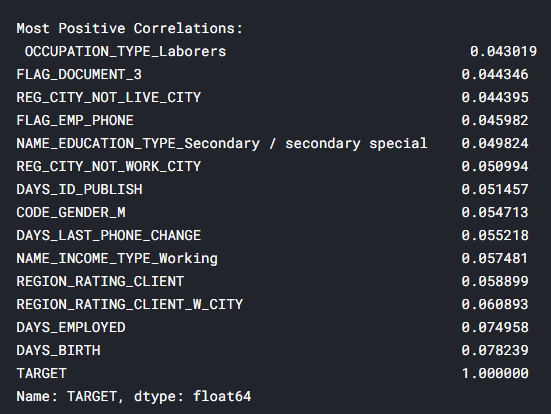
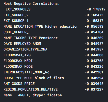
: DAYSBIRTH — ( TARGET, 1). , DAYSBIRTH — . , , , , , (.. == 0). , , .
app_train['DAYS_BIRTH'] = abs(app_train['DAYS_BIRTH'])
app_train['DAYS_BIRTH'].corr(app_train['TARGET'])
-0.07823930830982694
, , , , .
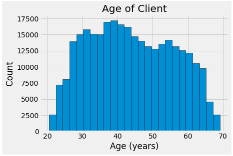
. -, . , x .
plt.style.use('fivethirtyeight')
#
plt.hist(app_train['DAYS_BIRTH'] / 365, edgecolor = 'k', bins = 25)
plt.title('Age of Client'); plt.xlabel('Age (years)'); plt.ylabel('Count');
, , , . , (KDE), . ( , , , ). seaborn kdeplot.
plt.figure(figsize = (10, 8))
sns.kdeplot(app_train.loc[app_train['TARGET'] == 0, 'DAYS_BIRTH'] / 365, label = 'target == 0')
sns.kdeplot(app_train.loc[app_train['TARGET'] == 1, 'DAYS_BIRTH'] / 365, label = 'target == 1')
plt.xlabel('Age (years)'); plt.ylabel('Density'); plt.title('Distribution of Ages');
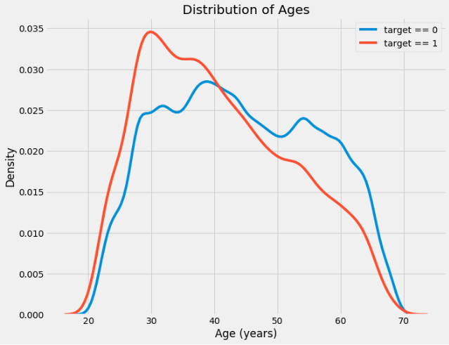
target == 1 . ( -0,07), , , , . : .
, 5 . , .
age_data = app_train[['TARGET', 'DAYS_BIRTH']]
age_data['YEARS_BIRTH'] = age_data['DAYS_BIRTH'] / 365
age_data['YEARS_BINNED'] = pd.cut(age_data['YEARS_BIRTH'], bins = np.linspace(20, 70, num = 11))
age_data.head(10)

#
age_groups = age_data.groupby('YEARS_BINNED').mean()
age_groups

plt.figure(figsize = (8, 8))
plt.bar(age_groups.index.astype(str), 100 * age_groups['TARGET'])
plt.xticks(rotation = 75); plt.xlabel('Age Group (years)'); plt.ylabel('Failure to Repay (%)')
plt.title('Failure to Repay by Age Group');

: . 10% 5% .
: , , . , , , .
: EXTSOURCE1, EXTSOURCE2 EXTSOURCE3. , « ». , , , , , .
.
-, EXT_SOURCE .
ext_data = app_train[['TARGET', 'EXT_SOURCE_1', 'EXT_SOURCE_2', 'EXT_SOURCE_3', 'DAYS_BIRTH']]
ext_data_corrs = ext_data.corr()
ext_data_corrs

plt.figure(figsize = (8, 6))
#
sns.heatmap(ext_data_corrs, cmap = plt.cm.RdYlBu_r, vmin = -0.25, annot = True, vmax = 0.6)
plt.title('Correlation Heatmap');
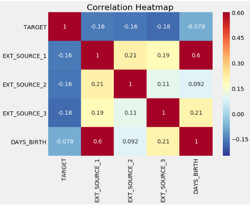
EXT_SOURCE , , EXT_SOURCE . , DAYS_BIRTH EXT_SOURCE_1, , , , .
, . .
plt.figure(figsize = (10, 12))
for i, source in enumerate(['EXT_SOURCE_1', 'EXT_SOURCE_2', 'EXT_SOURCE_3']):
plt.subplot(3, 1, i + 1)
sns.kdeplot(app_train.loc[app_train['TARGET'] == 0, source], label = 'target == 0')
sns.kdeplot(app_train.loc[app_train['TARGET'] == 1, source], label = 'target == 1')
plt.title('Distribution of %s by Target Value' % source)
plt.xlabel('%s' % source); plt.ylabel('Density');
plt.tight_layout(h_pad = 2.5)
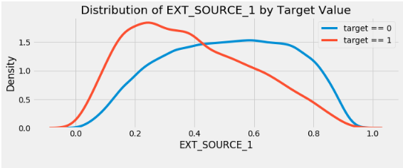
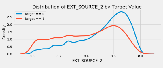
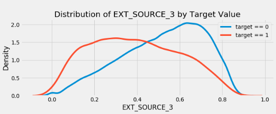
EXT_SOURCE_3 . , . ( ), , , .
EXTSOURCE DAYSBIRTH. – , , . seaborn PairGrid, , 2D .
plot_data = ext_data.drop(columns = ['DAYS_BIRTH']).copy()
plot_data['YEARS_BIRTH'] = age_data['YEARS_BIRTH']
plot_data = plot_data.dropna().loc[:100000, :]
#
def corr_func(x, y, **kwargs):
r = np.corrcoef(x, y)[0][1]
ax = plt.gca()
ax.annotate("r = {:.2f}".format(r),
xy=(.2, .8), xycoords=ax.transAxes,
size = 20)
#
grid = sns.PairGrid(data = plot_data, size = 3, diag_sharey=False,
hue = 'TARGET',
vars = [x for x in list(plot_data.columns) if x != 'TARGET'])
grid.map_upper(plt.scatter, alpha = 0.2)
grid.map_diag(sns.kdeplot)
grid.map_lower(sns.kdeplot, cmap = plt.cm.OrRd_r);
plt.suptitle('Ext Source and Age Features Pairs Plot', size = 32, y = 1.05);
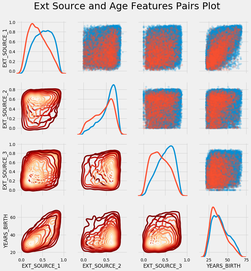
In this graph, red indicates loans that have not been repaid, and blue indicates loans that have been repaid. We can see various relationships in the data. There is indeed a moderate positive linear relationship between EXT_SOURCE_1 and YEARS_BIRTH, indicating that this trait may be age-specific.
This concludes the first article. In the next part, I will talk about developing additional features based on the available data, and also demonstrate how to create a simple machine learning model.
In preparing the article, materials from open sources were used: source_1 , source_2 .