Pure Cython VS nvc ++: burn metal plates to GPU for speed comparison

Let's heat metal plates on the GPU



Everyone knows that Python does not shine with speed by itself. In my opinion, the language is excellent in its readability, but the main niche of its application is where you wait most of the time for some data input / output. By convention, you can write super-performing code in Rust or C, but 99% of the time it will just wait.



However, Python is also great as a high-level syntactic glue. In this case, its leisurely interpreted part invokes high-speed code written in compiled programming languages. Typically, traditional libraries such as NumPy are used for this.



But we will go a little further, try to parallelize computations in CUDA and use a strange but working hybrid of C ++, stdpar and the nvc ++ compiler from Nvidia. Well, at the same time, let's try to evaluate the performance. Let's take two problems: sorting numbers and the Jacobi method, which we will use to calculate the heating of a metal plate.

Calling C ++ from Python

Our sorting code will look like this:

# distutils: language=c++
from libcpp.algorithm cimport sort

def cppsort(int[:] x):
    sort(&x[0], &x[-1] + 1)

      
      

        
        
        
      

    
        
        
        
      
      

        
        
        
      

    
    

In the first line, we explicitly indicate that Cython should use C ++, and not the default C. In the second, we import the sort function from C ++, and then the logic itself follows. Place the code in the cppsort.pyx file. Note that the extension is different from the usual py, as we will compile it or execute cythonize in Cython terminology.



Compilation can be done manually or included in setup.py, where we fully describe the preparation of our environment.



In setup.py, it looks like this:

from setuptools import setup
from Cython.Build import cythonize

setup(
    ext_modules = cythonize("cppsort.pyx")
)

      
      

        
        
        
      

    
        
        
        
      
      

        
        
        
      

    
    

But we can just do this on the command line:

cythonize -i cppsort.pyx

      
      

        
        
        
      

    
        
        
        
      
      

        
        
        
      

    
    

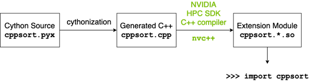
Under the hood, something like this will happen:

1. Cython will translate python code to C ++ and generate a valid cppsort.cpp.
2. C ++ compiler (in this case g ++) compiles C ++ code into Python extension module
3. The Python extension module is imported into the code as a regular Python module.

After compilation, we can import and immediately test the sorting:

from cppsort import cppsort
import numpy as np

x = np.array([4, 3, 2, 1], dtype="int32")
print(x)
cppsort(x)
print(x)

      
      

        
        
        
      

    
        
        
        
      
      

        
        
        
      

    
    

The array [4, 3, 2, 1] is successfully sorted to [1, 2, 3, 4] using C ++ std :: sort.

Let's go to the GPU?

C ++ standard library algorithms can be called with the parallel execution policy argument . This argument tells the compiler that you want to split the algorithm into parallel processes.



That being said, C ++ has several options for this policy:

1. std :: execution :: seq: Sequential execution. Parallelism is prohibited.
2. std :: execution :: unseq: Vectorized execution within the calling thread.
3. std :: execution :: par: Parallel execution on one or more threads.
4. std :: execution :: par_unseq: Parallel execution on one or more threads. Each stream will be vectorized whenever possible.

In this case, you yourself must monitor the race condition and deadlock. The standard g ++ compiler will try to distribute computation across CPU cores. But we can take a proprietary compiler from Nvidia - nvc ++ and feed it the "-stdpar" option. stdpar is Nvidia's C ++ Standard Parallelism with parallel code execution on the GPU.



Let's rewrite the code, taking into account the need to create a local copy of the array, since the GPU will not be able to access the array located within NumPy.

from libcpp.algorithm cimport sort, copy_n
from libcpp.vector cimport vector
from libcpp.execution cimport par

def cppsort(int[:] x):
    cdef vector[int] temp
    temp.resize(len(x))
    copy_n(&x[0], len(x), temp.begin())
    sort(par, temp.begin(), temp.end())
    copy_n(temp.begin(), len(x), &x[0])

      
      

        
        
        
      

    
        
        
        
      
      

        
        
        
      

    
    

Now this needs to be compiled again, but using nvc ++. This time, let's write a normal setup.py and call it:

CC=nvc++ python setup.py build_ext --inplace

      
      

        
        
        
      

    
        
        
        
      
      

        
        
        
      

    
    

We import into the code and try to call:

x = np.array([4, 3, 2, 1], dtype="int32")
cppsort(x) #     GPU

      
      

        
        
        
      

    
        
        
        
      
      

        
        
        
      

    
    

Performance

Traditionally, GPUs are good where there is a lot of the same type of lightweight computing. Heavy tasks, single GPU tasks will not work. Moreover, it is worth considering the volume of your data. If you have little data, then you will get a large overhead for the parallelization process, I / O between the CPU and GPU. As a result, such code will most likely run most efficiently on a bare CPU, sometimes even within a single core, if there is very little data. But on large arrays, the GPU will definitely be ahead.



There is a great comparison of sorting here. The NumPy speed was taken as a unit, and then the multiplicity of the speed increase in each method was calculated relative to it.









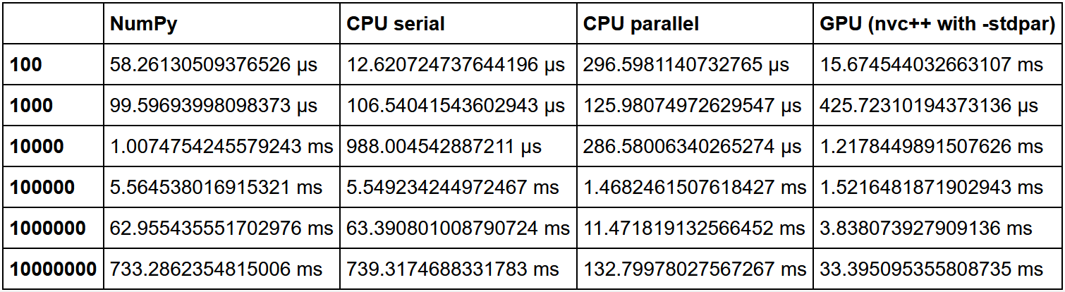
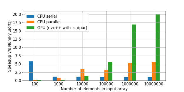
As we can see, the hypothesis that the gain in using the GPU on a large amount of data is growing is confirmed.

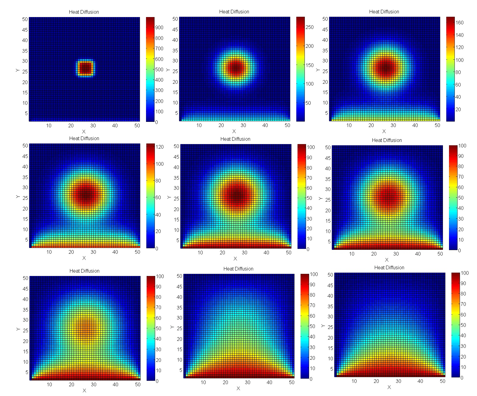
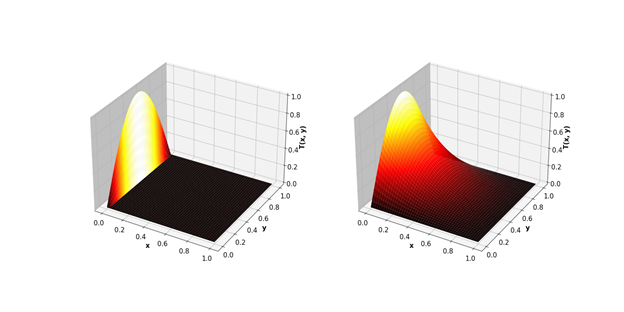
We calculate the heating of the plate

Let's take a problem closer to real engineering modeling - calculations using the Jacobi method. In particular, they are excellent for calculating temperature processes in 2D space.









Let's write a similar solver in Cython for subsequent compilation using CUDA:

# distutils: language=c++
# cython: cdivision=True
from libcpp.algorithm cimport swap
from libcpp.vector cimport vector
from libcpp cimport bool, float
from libc.math cimport fabs
from algorithm cimport for_each, any_of, copy
from execution cimport par, seq
 
cdef cppclass avg:
    float *T1
    float *T2
    int M, N
 
    avg(float* T1, float *T2, int M, int N):
        this.T1, this.T2, this.M, this.N = T1, T2, M, N
    inline void call "operator()"(int i):
        if (i % this.N != 0 and i % this.N != this.N-1):
            this.T2[i] = (
                this.T1[i-this.N] + this.T1[i+this.N] + this.T1[i-1] + this.T1[i+1]) / 4.0
cdef cppclass converged:
    float *T1
    float *T2
    float max_diff
 
    converged(float* T1, float *T2, float max_diff):
        this.T1, this.T2, this.max_diff = T1, T2, max_diff
 
    inline bool call "operator()"(int i):
        return fabs(this.T2[i] - this.T1[i]) > this.max_diff
 
def jacobi_solver(float[:, :] data, float max_diff, int max_iter=10_000):
    M, N  = data.shape[0], data.shape[1]
    cdef vector[float] local
    cdef vector[float] temp
    local.resize(M*N)
    temp.resize(M*N)
    cdef vector[int] indices = range(N+1, (M-1)*N-1)
    copy(seq, &data[0, 0], &data[-1, -1], local.begin())
    copy(par, local.begin(), local.end(), temp.begin())
    cdef int iterations = 0
    cdef float* T1 = local.data()
    cdef float* T2 = temp.data()
 
    keep_going = True
    while keep_going and iterations < max_iter:
        iterations += 1
        for_each(par, indices.begin(), indices.end(), avg(T1, T2, M, N))
        keep_going = any_of(par, indices.begin(), indices.end(), converged(T1, T2, max_diff))
        swap(T1, T2)
 
    if (T2 == local.data()):
        copy(seq, local.begin(), local.end(), &data[0, 0])
    else:
        copy(seq, temp.begin(), temp.end(), &data[0, 0])
    return iterations

      
      

        
        
        
      

    
        
        
        
      
      

        
        
        
      

    
    

As a result, the GPU gap is even more significant.

Minuses

1. Writing this kind of code is somewhat more complicated than a pure Python version and requires an understanding of how parallel computing works on a GPU.
2. It is required to copy the data into a separate array for transfer to the GPU, where the video card does not have access. This can be a problem when dealing with very large arrays.