🚚 🕐 🥅 Representative power constraints and generalization error estimation for graph neural networks 👐🏼 👴🏽 🚑

At present, one of the trends in the study of graph neural networks is the analysis of the operation of such architectures, comparison with nuclear methods, assessment of complexity and generalizing ability. All this helps to understand the weak points of existing models and creates space for new ones.

The work is aimed at investigating two problems related to graph neural networks. First, the authors give examples of graphs that are different in structure, but indistinguishable for both simple and more powerful GNNs . Second, they bound the generalization error for graph neural networks more accurately than VC bounds.

Introduction

Graph neural networks are models that work directly with graphs. They allow you to consider information about the structure. A typical GNN includes a small number of layers that are applied sequentially, updating the vertex representations at each iteration. Examples of popular architectures: GCN , GraphSAGE , GAT , GIN .

The process of updating vertex embeddings for any GNN architecture can be summarized by two formulas:

$a_v ^ {t + 1} = AGG \ left (h_w ^ t: w \ in \ mathcal {N} \ left (v \ right) \ right) \\ h_v ^ {t + 1} = COMBINE \ left (h_v ^ t, a_v ^ {t + 1} \ right),$

where AGG is usually a function invariant to permutations ( sum , mean , max etc.), COMBINE is a function that combines the representation of a vertex and its neighbors.

Computation tree for two-layer GNN using the example of node A. Source: https://eng.uber.com/uber-eats-graph-learning/

More advanced architectures may consider additional information such as edge features, edge angles, etc.

The article discusses the GNN class for the graph classification problem. These models are structured like this:

First, vertices are embeddings using L steps of graph convolutions
(, sum, mean, max)

GNN:

(LU-GNN). GCN, GraphSAGE, GAT, GIN
CPNGNN, , 1 d, d - ( port numbering)
DimeNet, 3D-,

LU-GNN

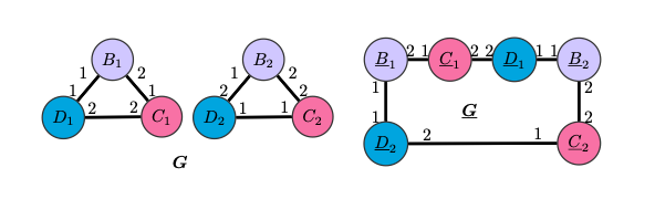
G G LU-GNN, , , readout-, . CPNGNN G G, .

CPNGNN

, “” , CPNGNN .

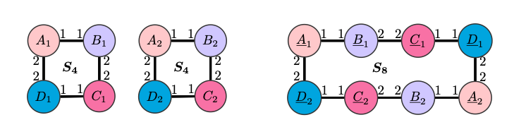
S₈ S₄ , , ( ), , , CPNGNN readout-, , . , .

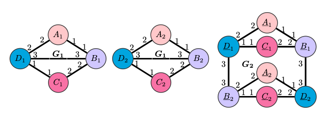
CPNGNN G₂ G₁. , DimeNet , , , , $\ angle A_1B_1C_1$ $\ angle \ underline {A} _1 \ underline {B} _1 \ underline {C} _1$ .

DimeNet

DimeNet G₄ , G₃, . , . , G₄ G₃ S₄ S₈, , , DimeNet S₄ S₈ .

GNN

. , , .

GNN, :

DimeNet
message- $m_ {uv} ^ {\ left (l \ right)}$ $\ Phi_ {uv}$ $\ underline {m} _ {uv} ^ {\ left (l \ right)} = \ underline {f} \ left (m_ {uv} ^ {\ left (l \ right)}, \ Phi_ {uv} \ right )$
$\ left (c_v \ left (i \ right), t_ {i, v} \ right)$ , c - i- v, t - .

:

$h_{v}^{\left( l + 1 \right)} = f \left( h_{v}^{\left( l \right)}, \underline{m}_{c_v\left( 1 \right)v}^{\left( l \right )}, t_{1, v}, ..., \underline{m}_{c_v\left( d \left( v \right ) \right)v}^{\left( l \right )}, t_{ d \left( v \right ), v} \right )$
readout-

: LU-GNN,

$h_v^{l + 1} = \phi \left( W_1x_v + W_2 \rho \left( \sum_{u \in \mathcal{N} \left( v \right)} g\left( h_u^l \right)\right) \right),$

$\phi,\ g,\ \rho$ - , x_v - v, , $\rho \left(0\right) = 0,\ \forall v: \lVert x_v \rVert_2 \le B_x,\ \forall x \in \mathbb{R}^r: \lVert \phi \left( x \right ) \rVert_{\infty} \le b < \infty,\ \phi\left( 0 \right ) = 0,\ g\left( 0 \right ) = 0$ . , $\phi,\ g,\ \rho$ $C_{\phi},\ C_{g},\ C_{\rho}$ , $\lVert W_1 \rVert_2 \le B_1,\ \lVert W_2 \rVert_2 \le B_2$ . $W_1,\ W_2,\ \phi,\ g,\ \rho$ GNN.

. $\beta$ $\lVert \beta \rVert_2 \le B_{\beta}$ .

$f\left(G\right)$ - GNN $y \in \{0, 1\}$ , $p \ left (f \ left (G \ right), y \ right) = y \ left (2f \ left (G \ right) - 1 \ right) + \ left (1 - y \ right) \ left (1 - 2 f \ left (G \ right) \ right)$ - , $p \ left (f \ left (G \ right), y \ right) <0$ .

, $a = -p \ left (f \ left (G \ right), y \ right)$ , $\ mathbb {I} \ left [\ right]$ - :

$loss _ {\ gamma} \ left (a \ right) = \ mathbb {I} \ left [a> 0 \ right] + (1 + \ frac {a} {\ gamma}) \ mathbb {I} \ left [a \ in \ left [\ gamma, 0 \ right] \ right].$

GNN $\ {G_j, y_j \} _ {j = 1} ^ m$ :

$\ hat {\ mathcal {R}} \ left (f \ right) = \ frac {1} {m} \ sum_ {j = 1} ^ m loss _ {\ gamma} \ left (-p \ left (f \ left (G_j \ right), y_j \ right) \ right)$

, , , , GNN . , (GNN, ), , , .

, :