, , “” — . , , , .
, .
3D ML :
GitHub .
IT- “VR/AR & AI” — PHYGITALISM.
?
, . , , , , , , .
, , , .
, “Representation Learning on Graphs: Methods and Applications” [1]. , Stanford CS224W: Machine Learning with Graphs. Sberloga, , , . ODS, (.. ).
Medium:
- How to do Deep Learning on Graphs with Graph Convolutional Networks Tobias Skovgaard Jepsen;
- - A Gentle Introduction to Graph Neural Networks (Basics, DeepWalk, and GraphSage) - Hands-on Graph Neural Networks with PyTorch & PyTorch Geometric Kung-Hsiang, Huang (Steeve);
- Jan H. Jensen ( );
- Medium — .
3D ML , , . — , (. [15]), , , (. [14]). , 3D ML, .
, , , ( python rdkit python NetworkX). , PyTorch Geometric ( , , ). TensorFlow Graphics “Semantic mesh segmentation”, , , . 3D ML .
, 4, , .
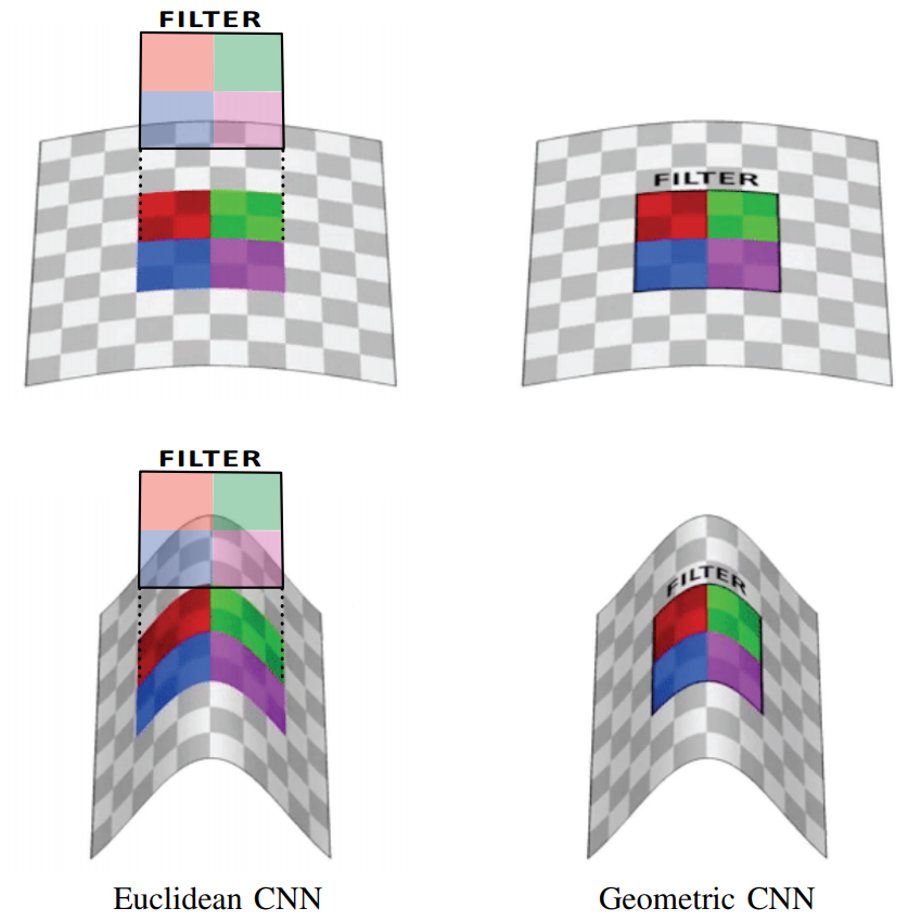
.1 [2]: , (Euclidean CNN) , , , (Geometric CNN, ).
— , “” () . , , ( ). , , , . , , .
, “Geometric deep learning: going beyond Euclidean data” [2] ( 3D ML, , ).
:
- (shift-invariance): (, ) , , . : .
- (locality): ( , ). , , .
- (compositionality or hierarchy): , , “ ” ( , : , , ..).
. — ( ).
, , ( ) ( ).

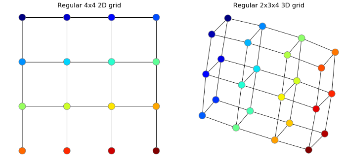
.2 : MNIST; : . (. [3]).
:
import networkx as nx

G = nx.grid_graph([4, 4])
nx.draw(G)
, .
, . , , — . (dot product) ( ), (. ). “A guide to convolution arithmetic for deep learning” [4].
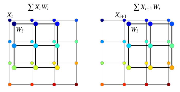
, , . , , , , .
, , , — ( , , 9 ). .. pooling . , , ,
, . , - .. “” . .

.3 [5].
. : — ( — , — ), — . , ( ) , — .
- , , . — (averaging) [6] (summation) [7] , . , . [8].
5 (.4). :
, , , , .

.4
.
“” . , . , .
, ( MNIST). — - , — - . :
, ( ), , MNIST , 91% ( ).
, ( — ). — . . , .
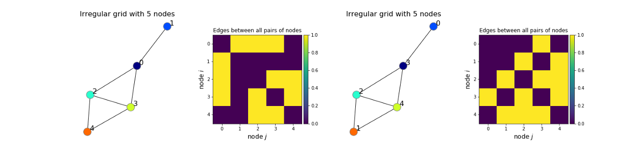
.5 5 ( — 0, — 1) .
, MNIST. numpy:
import numpy as np
from scipy.spatial.distance import cdist
img_size = 28  # MNIST image width and height
col, row = np.meshgrid(np.arange(img_size), np.arange(img_size))
coord = np.stack((col, row), axis=2).reshape(-1, 2) / img_size
dist = cdist(coord, coord)  # . 6 ( )
sigma = 0.2 * np.pi  # width of a Gaussian
A = np.exp(-dist ** 2 / sigma ** 2) # .6 (  )
, dist
—
,
— ( , , ). , , — , (. [2, 9]).
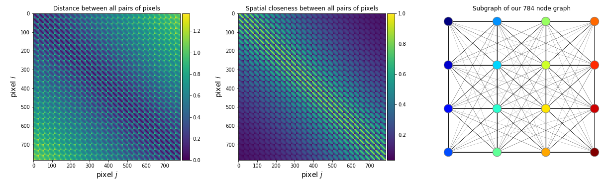
.6 -: , ,
.
, , .. . , :
- [7];
- [6].
, , :
, .
PyTorch, :
import torch
import torch.nn as nn

C = 2  # Input feature dimensionality
F = 8  # Output feature dimensionality
W = nn.Linear(in_features=C, out_features=F)  # Trainable weights

# Fully connected layer
X = torch.randn(1, C)  # Input features
Z = W(X)  # Output features : torch.Size([1, 8])

#Graph Neural Network layer
N = 6  # Number of nodes in a graph
X = torch.randn(N, C)  # Input feature
A = torch.rand(N, N)  # Adjacency matrix (edges of a graph)
Z = W(torch.mm(A, X))  # Output features: torch.Size([6, 8])
. , MNIST , , . , , , , , , , . , , [10, 11, 12].
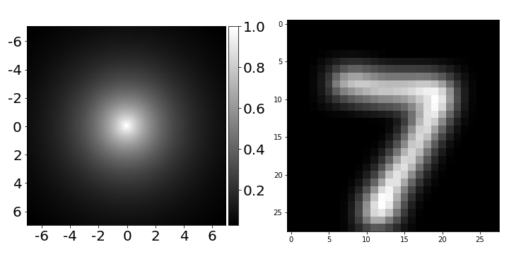
.7 , , () ().
, , :
import torch.nn as nn           # using PyTorch
nn.Sequential(nn.Linear(4, 64), # map coordinates to a hidden layer
             nn.ReLU(),         # nonlinearity
             nn.Linear(64, 1),  # map hidden representation to edge
             nn.Tanh())         # squash edge values to [-1, 1]

.8 2D- , , . (, 92,24%), (, 91,05%), (, 92,39%).
import imageio  # to save GIFs
import matplotlib as mpl
import matplotlib.pyplot as plt
import numpy as np
from scipy.spatial.distance import cdist
import cv2  # optional (for resizing the filter to look better)

img_size = 28
# Create/load some adjacency matrix A (for example, based on coordinates)
col, row = np.meshgrid(np.arange(img_size), np.arange(img_size))
coord = np.stack((col, row), axis=2).reshape(-1, 2) / img_size
dist = cdist(coord, coord)  # distances between all pairs of pixels
sigma = 0.2 * np.pi  # width of a Gaussian (can be a hyperparameter when training a model)

A = np.exp(- dist / sigma ** 2)  # adjacency matrix of spatial similarity
# above, dist should have been squared to make it a Gaussian (forgot to do that)

scale = 4
img_list = []
cmap = mpl.cm.get_cmap('viridis')
for i in np.arange(0, img_size, 4):  # for every row with step 4
    for j in np.arange(0, img_size, 4):  # for every col with step 4
        k = i*img_size + j
        img = A[k, :].reshape(img_size, img_size)
        img = (img - img.min()) / (img.max() - img.min())
        img = cmap(img)
        img[i, j] = np.array([1., 0, 0, 0])  # add the red dot
        img = cv2.resize(img, (img_size*scale, img_size*scale))
        img_list.append((img * 255).astype(np.uint8))
imageio.mimsave('filter.gif', img_list, format='GIF', duration=0.2)
, , ( ), . , , : , , , . (, , ), , [13].
(GNN) — , . , . GNN — . , GNN .

.9 GNN “Anisotropic, Dynamic, Spectral and Multiscale Filters Defined on Graphs”.
, .
, , [6].
, Medium.
- Hamilton, WL, Ying, R. and Leskovec, J., 2017. Representation learning on graphs: Methods and applications. arXiv preprint arXiv: 1709.05584. [ paper ]
- Bronstein, MM, Bruna, J., LeCun, Y., Szlam, A. and Vandergheynst, P., 2017. Geometric deep learning: going beyond euclidean data. IEEE Signal Processing Magazine, 34 (4), pp. 18-42. [ paper ]
- Fey, M., Eric Lenssen, J., Weichert, F. and Müller, H., 2018. Splinecnn: Fast geometric deep learning with continuous b-spline kernels. In Proceedings of the IEEE Conference on Computer Vision and Pattern Recognition (pp. 869-877). [paper]
- Dumoulin, V. and Visin, F., 2016. A guide to convolution arithmetic for deep learning. arXiv preprint arXiv:1603.07285. [paper]
- Achanta, R., Shaji, A., Smith, K., Lucchi, A., Fua, P. and Süsstrunk, S., 2012. SLIC superpixels compared to state-of-the-art superpixel methods. IEEE transactions on pattern analysis and machine intelligence, 34(11), pp.2274-2282. [paper]
- Kipf, T.N. and Welling, M., 2016. Semi-supervised classification with graph convolutional networks. arXiv preprint arXiv:1609.02907. [paper]
- Xu, K., Hu, W., Leskovec, J. and Jegelka, S., 2018. How powerful are graph neural networks?.. arXiv preprint arXiv:1810.00826. [paper]
- Hamilton, W., Ying, Z. and Leskovec, J., 2017. Inductive representation learning on large graphs. In Advances in neural information processing systems (pp. 1024-1034). [paper]
- Defferrard, M., Bresson, X. and Vandergheynst, P., 2016. Convolutional neural networks on graphs with fast localized spectral filtering. Advances in neural information processing systems, 29, pp.3844-3852. [paper]
- Jia, X., De Brabandere, B., Tuytelaars, T. and Gool, L.V., 2016. Dynamic filter networks. In Advances in neural information processing systems (pp. 667-675). [paper]
- Simonovsky, M. and Komodakis, N., 2017. Dynamic edge-conditioned filters in convolutional neural networks on graphs. In Proceedings of the IEEE conference on computer vision and pattern recognition (pp. 3693-3702). [paper]
- Knyazev, B., Lin, X., Amer, M.R. and Taylor, G.W., 2018. Spectral multigraph networks for discovering and fusing relationships in molecules. arXiv preprint arXiv:1811.09595. [paper]
- Knyazev, B., Lin, X., Amer, M.R. and Taylor, G.W., 2019. Image classification with hierarchical multigraph networks. arXiv preprint arXiv:1907.09000. [paper]
- Wang, Y., Sun, Y., Liu, Z., Sarma, S.E., Bronstein, M.M. and Solomon, J.M., 2019. Dynamic graph cnn for learning on point clouds. Acm Transactions On Graphics (tog), 38(5), pp.1-12. [paper]
- Verma, N., Boyer, E. and Verbeek, J., 2018. Feastnet: Feature-steered graph convolutions for 3d shape analysis. In Proceedings of the IEEE conference on computer vision and pattern recognition (pp. 2598-2606). [paper]