
I have participated in exercises with the Company Risk Matrix.
The action took place in three stages. The first one: boys and girls were questioned with questions like “have you stopped drinking cognac in the morning”, to which you only need to answer “yes” or “no”.
At the second stage, a “science-based” risk matrix was shown.
At the permanent third stage, all the divisions of that company tried from year to year to move to lower positions on the matrix, but this was possible only due to personal charm. Those who could not move became extreme on any business failure.
1. Risk matrix: it is convenient to fill in, it is not convenient to work.
Here is a typical Risk Matrix that Google offers.

For example, a random Risk Matrix from a very old report was found on the Internet.
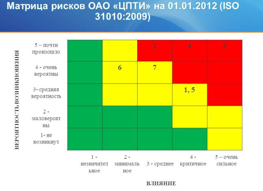
The numbers inside the colored rectangles represent meaningful risk interpretations that are not really needed yet. The description of the risk is very broad and vague. It is hard to believe that all the components of the description, separately and together, give a single number in a very narrow range.
If you follow the typical Google matrix, then all meaningful descriptions of "probability" and "impact" can be associated with specific numbers.
Here is a template of a modernized Google matrix with multiplied probabilities corresponding to horizontal and vertical scaling.

It is not very convenient for using standard matrix operations, since it is symmetric with respect to the additional, not the main, diagonal.
It is possible that the Risk Matrix in this form is more convenient for managers. Its rearrangement with symmetry about the main diagonal does not change the essence of the matrix. Alternatively, you can always step back and go back to the original view.
The matrix is rebuilt by replacing the row order with the opposite (symmetry about the vertical central axis). As a result, a matrix is obtained that is symmetric about the main diagonal.

The same transformations for the studied Risk Matrix.

Numbers other than 0 are the risk number associated with a certain structural unit. This encoding only takes place in connection with the bureaucratic hierarchy in the company, and not with the risks. For example, for the element {1,5}. In terms of risk, the situation is no different if the descriptions of risk1 and risk5 are combined. If these are different risks, then you can reduce the matrix step and place the risk in a more appropriate position.
Ultimately, transformations should make each different risk a separate element.
Position [1,3] in the standard matrix numbering system means the element at the intersection of the 1st row and 3rd column. For the matrix under consideration, in position [1,3] is the number 2. This means that if there is a scale with the maximum value “5 - almost happened” (1.), then in [1,3] we expect “3 - average” ( 0.6) influence. Let the “influence” in the scaled interval correspond to a certain damage: 5-d5, 4-d4, 3-d3, 2-d2,1-d1. Then, if during a certain period there was 1 accident from group 2, then the damage will be 1. * 0.6 * d3 * 1, and if n accidents from group 2 occurred during the same period, then the damage will be 1. * 0.6 * d3 * n
Then the investigated matrix will take the form.

Another transformation is carried out: transposition by changing the positions of columns and rows.

The bottom row of the legend becomes redundant, since the corresponding probability is taken into account in the matrix values. The first vertical column is also taken into account in the values of the matrix, but it is important because it sets the structure of events that can be recorded or predicted over a certain period. Having a column vector from the number of events related to the corresponding type (very strong, critical, ...), you can multiply the matrix by a column vector in a standard way and get a structured amount of damage.
Without the legend, the matrix will look like this.

2. Risk matrix: it is convenient to calculate, not convenient to analyze.
The first main task.
Having received the matrix A, one can proceed to solving the first main problem: with a known number and quality of the events that have occurred, calculate the amount of damage.
Let for a certain period 2 "very strong" events occurred, 3 "critical", 1 "average", 5 "minimal" and 7 "insignificant". Multiplying the matrix A by the vector of the number of events, we obtain the damage structure.

General damage.

Now you can check the accuracy of estimates, make adjustments, evaluate possible options for reducing the amount of damage.
The above transformations of the original matrix were carried out to obtain a simple computational damage procedure. From matrix A, you can always return unambiguously to the original matrix.
3. Risk matrix: what theory is behind it?
For any non-degenerate square matrix, there is a one-to-one linear transformation corresponding to this matrix. When looking at a matrix, it is difficult to understand which linear transformation is behind it. In addition, it is not known in what basis the matrix representation is produced.
The risk matrix is a square matrix and must correspond to some kind of linear transformation. This fact does not depend on the method of obtaining the matrix and the ideas implemented in a specific method for obtaining the matrix.
It is important that the determinant of the matrix is not zero. These are requirements of a method that provides a canonical representation of a matrix.
Further, it is shown that this is not just a limitation of the method, but a requirement that meets the needs of practice.
The considered Risk Matrix has two zero rows and one zero column. In any case, the determinant of this matrix will be equal to zero. Below is a graphic showing how the company intends to mitigate risks.

The arrows show how the risks will be reduced. It doesn't matter how it is, it is important that the new situation is again represented as a matrix. Some linear transformation corresponds to this matrix. The transition from the “old” matrix to the “new” one is a matrix and a linear transformation.
What does a nonzero determinant mean? This is the ability to walk back and forth. If the determinant is zero, then the step "back" cannot be done.
At the same time, the risk reduction matrix is initially associated with the “old” matrix. That is, in the picture you can and should hover "back and forth", but in the formalized version you cannot walk "back and forth".
The next problem is related to the fact that a large risk with a low probability can be compared with the risk from a very large number of small risks with a low probability.
In the above example, the 7 minor events do not formally cause any damage. It is clear that this is not the case. The absence of small risks only emphasizes the insufficient incorrectness of the formation of the Risk Matrix.
Let the determinant of the Risk Matrix be not equal to zero and this is a consequence of the continuity of work to reduce risks, and not an artificial requirement of the mathematical method for business.
So, there are:
- Risk matrix, which corresponds to an unknown linear transformation and an unknown basis;
- the determinant of the Matrix, which is not equal to zero.
What can be done? Bring the Risk Matrix to a canonical form with an understandable orthonormal basis.
In the work of Alexander Emelin, the following allegorical description of the advantages of the canonical form is given. “Suppose there is a piece of paper with a word written on it. But it is so complicated that the words cannot be seen. After the canonical transformation, the sheet is unfolded in such a way that the word can be seen. If an orthonormal basis is used, the piece of paper will remain the same size. ”
None of the operations and transformations described in the work change the essence of the phenomena reflected and contained in the Risk Matrix.
4. Risk matrix as an algebraic construction.
The second main task. Canonical representation.
Elements are added to the matrix under consideration so that the determinant is not equal to zero. Values are rounded to avoid formulas that are too large.

Further, according to the standard scheme, the matrix is reduced to the canonical form.
Eigenvalues of the Risk Matrix.

Further work with symbolic values will be difficult during orthogonalization and the result will be impossible to visualize (very cumbersome symbolic matrices).
Let (for example) d1 = 1, d2 = 2, d3 = 5, d4 = 8, d5 = 12.
Then the Risk Matrix M in the symmetric representation takes the form.

It is checked that the determinant is not equal to zero.
Eigenvalues are calculated.

A matrix of eigenvectors is found.

It is orthogonalized. This is the ORT matrix of orthonormal vectors.

To check, the first vector (column) is multiplied in pairs by all the others. The values are nonzero, but close to 0.

The new basis contains the representation of the original linear transformation (defining the Risk Matrix) in the variables z1, z2, z3, z4, z5.

If we neglect very small terms, then the canonical representation of the linear transformation is obtained.

Moreover, the coefficients at the squares correspond to the previously calculated eigenvalues.
New view of the Risk Matrix in an orthonormal basis.

It turns out an alternating quadratic form.
5. Practical use of the canonical representation.
What about the original Risk Matrix?
It represents an unknown linear transformation.
Its lines are designated (from top to bottom) as x1, x2, x3, x4, x5. The rows of the Risk Matrix represent the decomposition in an unknown basis.
So
x1 = 10 * d5 * b1 + 0 * b2 + 0 * b3 + 0 * b4 + 0 * b5,
x2 = 8 * d4 * b1 + 0 * b2 + 4 * d4 * b3 + 0 * b4 + 0 * b5 , etc.
The presence of an orthonormal basis provides freedom of movement between the variables X and Z.
In the variables Z, the linear transformation function in the orthonormal basis is clearly visible. The behavior of this same linear transformation in the original Risk Matrix was not clear.
The clear benefit of the canonical view is the ability to adjust the threat type. If initially the classification went in steps of 20%, now it can be revised by recalculating the values of the ends of the ranges in a new basis. There will also be 5 types of events, but the steps between them will be different.
A clear benefit of the canonical view is the ability to adjust the scaling for different types of events (incidents). If initially the scaling of events (very strong, critical, ...) went in steps of 20%, now it can be revised by recalculating the values of the ends of the ranges in a new basis. There will also be 5 types of events (incidents), but the steps between them will be different.
6. Risk Matrix: The quadratic form defines the content.
The described practical benefits may seem ridiculous against the background of the not quite simple manipulations done before: "the game is not worth the candle."
The clear, straightforward and simple form of the Google Risk Matrix does not quite match the content of risk management.
What is risk: you count on one thing, but in fact you get another.
Google's risk matrix is designed in such a way that the company always clearly knows its risks and consistently works to reduce them. Moreover, all high risks with great damage are gradually eliminated. Kudos to wise managers.
On the contrary, the Risk Matrix obtained in the orthonormal basis will always show the presence of non-empty high risks.
The canonical representation formed in Section 4 can be interpreted as the damage that occurs when the events that are expected occur: the variable in the square.
There is one more important circumstance. Damage also occurs if costs are made to prevent situations that do not occur.
Next new design.

The values v [i, j] correspond to the damage (benefit) provided that we were counting on the event f (j), but the event f (i) actually happened. The v [i, j] values can be either positive (harm) or negative (benefit).
The value v [i, i] corresponds to a situation when the event for which we were preparing actually happened: what we expected was what we got.
In this case, the Risk Matrix takes the form.

The column vector of events has the form.

In this case, the amount of damage is described by a quadratic form.

The presented new construction of the description of risks can be associated with the following calculations: assessment of damage in the actual occurrence of the event f (i), while the activities are focused on the event f (j).
Then it becomes clear what “risk mitigation measures” are required:
- for those risks that were not prepared for, but they often appear;
- for risks identified as basic.
In addition, all the algebraic manipulations described above become not only appropriate, but mandatory.
The problem of minimizing risks is reduced to minimizing the value of damage given by the canonical representation of the quadratic form of damage.
7. Risk matrix as a digital management tool.
In the general case, you can use different methods of risk assessment and management: simulation, queuing systems, assessment of the stability of structural schemes of serial-parallel connection of components, and others.
In this case, the "genre" of risk matrices and its opportunities for business improvement are considered.
In fact, the new form allows the Risk Matrix to move away from the role of a "bogeyman" and become a normal tool for digital business management. One of the many for today's business.
For this, it is necessary to change the methodology for calculating damage, focusing on verifiable quantitative values versus focusing on qualitative expert assessments.