For a long time I have not written any articles and, I think, it's time to write about there, how the knowledge in data science, obtained during the training of the well-known specialization from Yandex and MIPT “Machine Learning and Data Analysis”, came in handy. True, in fairness, it should be noted that knowledge has not been fully obtained - the specialty is not completed :) However, it is already possible to solve simple real business problems. Or is it necessary? This question will be answered in just a couple of paragraphs.
So, today in this article I will tell the dear reader about my first experience of participating in an open competition. I would like to note right away that my goal of the competition was not to get any prizes. The only desire was to try my hand in the real world :) Yes, in addition it so happened that the topic of the competition practically did not intersect with the material from the courses passed. This added some complications, but with that the competition became even more interesting and valuable the experience gained from there.
By tradition, I will designate who may be interested in the article. Firstly, if you have already completed the first two courses of the above specialization, and want to try your hand at practical problems, but are shy and worried that it may not work out and you will be laughed at, etc. After reading the article, such fears, I hope, will be dispelled. Secondly, perhaps you are solving a similar problem and do not know at all where to enter. And here is a ready-made unpretentious, as real datasinters say, a baseline :)
Here it would be worthwhile to outline the research plan, but we will digress a little and try to answer the question from the first paragraph - whether a beginner in datasinting needs to try his hand at such competitions. Opinions differ on this score. Personally, my opinion is necessary! Let me explain why. There are many reasons, I will not list everything, I will indicate the most important ones. Firstly, such competitions help to consolidate theoretical knowledge in practice. Secondly, in my practice, almost always, the experience gained in conditions close to combat, very strongly motivates for further exploits. Thirdly, and this is the most important thing - during the competition you have the opportunity to communicate with other participants in special chats, you don't even have to communicate, you can just read what people write about and this a) often leads to interesting thoughts aboutwhat other changes to make in the study; and b) gives confidence to validate their own ideas, especially if they are expressed in the chat. These advantages must be approached with a certain prudence, so that there is no feeling of omniscience ...
Now a little about how I decided to participate. I learned about the competition just a few days before it started. The first thought is “well, if I knew about the competition a month ago, I would have prepared myself, but I would have studied some additional materials that could be useful for conducting research, otherwise, without preparation, I can not meet the deadline ...”, the second the thought “actually, what might not work if the goal is not a prize, but participation, especially since the participants in 95% of cases speak Russian, plus there are special chats for discussion, there will be some kind of webinars from the organizers. In the end, it will be possible to see live data scientists of all stripes and sizes ... ". As you guessed, the second thought won, and it was not in vain - just a few days of hard work and I got a valuable experience, albeit a simple one,but quite a business task. Therefore, if you are on the way to conquering the heights of data science and see the upcoming competition, yes in your native language, with support in chats and you have free time - do not hesitate for a long time - try and may the force come with you! On a positive note, we move on to the task and research plan.
Matching names
We will not torture ourselves and come up with a description of the problem, but we will give the original text from the website of the competition organizer.
A task
When looking for new clients, SIBUR has to process information on millions of new companies from various sources. At the same time, company names may have different spellings, contain abbreviations or errors, and be affiliated with companies already known to SIBUR.
To process information about potential customers more efficiently, SIBUR needs to know if the two names are related (i.e. belong to the same company or affiliated companies).
In this case, SIBUR will be able to use already known information about the company itself or about affiliated companies, not duplicate calls to the company or not waste time on irrelevant companies or subsidiaries of competitors.
The training sample contains pairs of names from different sources (including custom ones) and markup.
The markup was obtained partly by hand, partly - algorithmically. In addition, the markup may contain errors. You are going to build a binary model that predicts whether two names are related. The metric used in this task is F1.
In this task, it is possible and even necessary to use open data sources to enrich the dataset or find additional information important for identifying affiliated companies.
Additional information about the task
Uncover me for more information
, . , : , , Sibur Digital, , Sibur international GMBH , “ International GMBH” .
: , .
, , , .
(50%) (50%) .
. , , .
1 1 000 000 .
( ). , .
24:00 6 2020 # .
, , , .
, , - , .
.
, , .
10 .
API , , 2.
“” crowdsource . , :)
, .
legel entities, , .. , Industries .
. .
, . , “” .
, , , . , , .
, , .
open source , . — . .
, - – . , , - , , , .
: , .
, , , .
(50%) (50%) .
. , , .
1 1 000 000 .
( ). , .
24:00 6 2020 # .
, , , .
, , - , .
.
, , .
10 .
API , , 2.
, , , .. crowdsource
“” crowdsource . , :)
, .
legel entities, , .. , Industries .
. .
, . , “” .
, , , . , , .
, , .
open source
open source , . — . .
, - – . , , - , , , .
Data
train.csv - training set
test.csv - test set
sample_submission.csv - example of a solution in the correct format
Naming baseline.ipynb - code
baseline_submission.csv - basic solution
Please note that the organizers of the competition took care of the younger generation and posted a basic solution to the problem, which gives an f1 quality of about 0.1. This is the first time I participate in a competition and the first time I see this :)
So, having familiarized ourselves with the problem itself and the requirements for its solution, let's move on to the solution plan.
Problem solving plan
Setting up technical instruments
Let's load the libraries
Let's write auxiliary functions
Data preprocessing
… -. !
50 & Drop it smart.
Let's calculate the Levenshtein distance
Calculate the normalized Levenshtein distance
Visualize the features
Compare the words in the text for each pair and generate a large bunch of features
Compare the words from the text with words from the names of the top 50 holding brands in the petrochemical and construction industries. Let's get the second big bunch of features. Second CHIT
Preparing data for feeding into the model
Setting up and training the model
Results of the competition
Sources of information
Now that we have familiarized ourselves with the research plan, let's move on to its implementation.
Setting up technical instruments
Loading Libraries
Actually, everything is simple here, first we will install the missing libraries
Install the library to determine the list of countries and then remove them from the text
pip install pycountry
Install a library for determining the Levenshtein distance between words from text with each other and with words from different lists
pip install strsimpy
We will install the library with the help of which we will transliterate the Russian text into Latin
pip install cyrtranslit
Pull up libraries
import pandas as pd
import numpy as np

import warnings
warnings.filterwarnings('ignore')

import pycountry
import re

from tqdm import tqdm
tqdm.pandas()

from strsimpy.levenshtein import Levenshtein
from strsimpy.normalized_levenshtein import NormalizedLevenshtein

import matplotlib.pyplot as plt
from matplotlib.pyplot import figure

import seaborn as sns
sns.set()
sns.set_style("whitegrid")

from sklearn.model_selection import train_test_split
from sklearn.model_selection import StratifiedKFold
from sklearn.model_selection import StratifiedShuffleSplit

from scipy.sparse import csr_matrix

import lightgbm as lgb
from sklearn.linear_model import LogisticRegression

from sklearn.metrics import accuracy_score
from sklearn.metrics import recall_score
from sklearn.metrics import precision_score
from sklearn.metrics import roc_auc_score

from sklearn.metrics import classification_report, f1_score


# import googletrans
# from googletrans import Translator
import cyrtranslit
Let's write auxiliary functions
It is considered good practice to specify the function in one line instead of copying a large piece of code. We will do so, almost always.
I won't argue that the quality of the code in the functions is excellent. In some places it should definitely be optimized, but in order to quickly research it, only the accuracy of the calculations will be enough.
So the first function converts the text to lowercase
The code
# convert text to lowercase
def lower_str(data,column):
    data[column] = data[column].str.lower()
The following four functions help to visualize the space of the features under study and their ability to separate objects by target labels - 0 or 1.
The code
# statistic table for analyse float values (it needs to make histogramms and boxplots)
def data_statistics(data,analyse,title_print):

    data0 = data[data['target']==0][analyse]
    data1 = data[data['target']==1][analyse]

    data_describe = pd.DataFrame()
    data_describe['target_0'] = data0.describe()
    data_describe['target_1'] = data1.describe()
    data_describe = data_describe.T

    if title_print == 'yes':
        print ('\033[1m' + '   ',analyse,'\033[m')
    elif title_print == 'no':
        None

    return data_describe

# histogramms for float values
def hist_fz(data,data_describe,analyse,size):
    print ()
    print ('\033[1m' + 'Information about',analyse,'\033[m')
    print ()

    data_0 = data[data['target'] == 0][analyse]
    data_1 = data[data['target'] == 1][analyse]

    min_data = data_describe['min'].min()
    max_data = data_describe['max'].max()

    data0_mean = data_describe.loc['target_0']['mean']
    data0_median = data_describe.loc['target_0']['50%']
    data0_min = data_describe.loc['target_0']['min']
    data0_max = data_describe.loc['target_0']['max']
    data0_count = data_describe.loc['target_0']['count']


    data1_mean = data_describe.loc['target_1']['mean']
    data1_median = data_describe.loc['target_1']['50%']
    data1_min = data_describe.loc['target_1']['min']
    data1_max = data_describe.loc['target_1']['max']
    data1_count = data_describe.loc['target_1']['count']


    print ('\033[4m' + 'Analyse'+ '\033[m','No duplicates')

    figure(figsize=size)
    sns.distplot(data_0,color='darkgreen',kde = False)

    plt.scatter(data0_mean,0,s=200,marker='o',c='dimgray',label='Mean')
    plt.scatter(data0_median,0,s=250,marker='|',c='black',label='Median')
    plt.legend(scatterpoints=1,
               loc='upper right',
               ncol=3,
               fontsize=16)
    plt.xlim(min_data, max_data)
    plt.show()
    print ('Quantity:', data0_count,
           '         Min:', round(data0_min,2),
           '         Max:', round(data0_max,2),
           '         Mean:', round(data0_mean,2),
           '         Median:', round(data0_median,2))

    print ()
    print ('\033[4m' + 'Analyse'+ '\033[m','Duplicates')

    figure(figsize=size)
    sns.distplot(data_1,color='darkred',kde = False)
    plt.scatter(data1_mean,0,s=200,marker='o',c='dimgray',label='Mean')
    plt.scatter(data1_median,0,s=250,marker='|',c='black',label='Median')
    plt.legend(scatterpoints=1,
               loc='upper right',
               ncol=3,
               fontsize=16)
    plt.xlim(min_data, max_data)
    plt.show()
    print ('Quantity:', data_1.count(),
           '         Min:', round(data1_min,2),
           '         Max:', round(data1_max,2),
           '         Mean:', round(data1_mean,2),
           '         Median:', round(data1_median,2))

# draw boxplot
def boxplot(data,analyse,size):
    print ('\033[4m' + 'Analyse'+ '\033[m','All pairs')

    data_0 = data[data['target'] == 0][analyse]
    data_1 = data[data['target'] == 1][analyse]

    figure(figsize=size)
    sns.boxplot(x=analyse,y='target',data=data,orient='h',
                showmeans=True,
                meanprops={"marker":"o",
                           "markerfacecolor":"dimgray",
                           "markeredgecolor":"black",
                          "markersize":"14"},
               palette=['palegreen', 'salmon'])
    plt.ylabel('target', size=14)
    plt.xlabel(analyse, size=14)
    plt.show()

# draw graph for analyse two choosing features for predict traget label
def two_features(data,analyse1,analyse2,size):
    fig = plt.subplots(figsize=size)

    x0 = data[data['target']==0][analyse1]
    y0 = data[data['target']==0][analyse2]
    x1 = data[data['target']==1][analyse1]
    y1 = data[data['target']==1][analyse2]

    plt.scatter(x0,y0,c='green',marker='.')
    plt.scatter(x1,y1,c='black',marker='+')
    plt.xlabel(analyse1)
    plt.ylabel(analyse2)
    title = [analyse1,analyse2]
    plt.title(title)
    plt.show()
The fifth function is designed to generate a guess and error table of the algorithm, better known as a conjugation table.
In other words, after the formation of the vector of forecasts, we need to compare the forecast with target labels. The result of such a comparison should be a conjugation table for each pair of companies from the training sample. In the conjugation table for each pair, the result of matching the forecast to the class from the training sample will be determined. Matching classification is accepted as follows: 'True positive', 'False positive', 'True negative' or 'False negative'. These data are very important for analyzing the operation of the algorithm and making decisions on improving the model and feature space.
The code
def contingency_table(X,features,probability_level,tridx,cvidx,model):
    tr_predict_proba = model.predict_proba(X.iloc[tridx][features].values)
    cv_predict_proba = model.predict_proba(X.iloc[cvidx][features].values)

    tr_predict_target = (tr_predict_proba[:, 1] > probability_level).astype(np.int)
    cv_predict_target = (cv_predict_proba[:, 1] > probability_level).astype(np.int)

    X_tr = X.iloc[tridx]
    X_cv = X.iloc[cvidx]

    X_tr['predict_proba'] = tr_predict_proba[:,1]
    X_cv['predict_proba'] = cv_predict_proba[:,1]

    X_tr['predict_target'] = tr_predict_target
    X_cv['predict_target'] = cv_predict_target

    # make true positive column
    data = pd.DataFrame(X_tr[X_tr['target']==1][X_tr['predict_target']==1]['pair_id'])
    data['True_Positive'] = 1
    X_tr = X_tr.merge(data,on='pair_id',how='left')

    data = pd.DataFrame(X_cv[X_cv['target']==1][X_cv['predict_target']==1]['pair_id'])
    data['True_Positive'] = 1
    X_cv = X_cv.merge(data,on='pair_id',how='left')

    # make false positive column
    data = pd.DataFrame(X_tr[X_tr['target']==0][X_tr['predict_target']==1]['pair_id'])
    data['False_Positive'] = 1
    X_tr = X_tr.merge(data,on='pair_id',how='left')

    data = pd.DataFrame(X_cv[X_cv['target']==0][X_cv['predict_target']==1]['pair_id'])
    data['False_Positive'] = 1
    X_cv = X_cv.merge(data,on='pair_id',how='left')

    # make true negative column
    data = pd.DataFrame(X_tr[X_tr['target']==0][X_tr['predict_target']==0]['pair_id'])
    data['True_Negative'] = 1
    X_tr = X_tr.merge(data,on='pair_id',how='left')

    data = pd.DataFrame(X_cv[X_cv['target']==0][X_cv['predict_target']==0]['pair_id'])
    data['True_Negative'] = 1
    X_cv = X_cv.merge(data,on='pair_id',how='left')

    # make false negative column
    data = pd.DataFrame(X_tr[X_tr['target']==1][X_tr['predict_target']==0]['pair_id'])
    data['False_Negative'] = 1
    X_tr = X_tr.merge(data,on='pair_id',how='left')

    data = pd.DataFrame(X_cv[X_cv['target']==1][X_cv['predict_target']==0]['pair_id'])
    data['False_Negative'] = 1
    X_cv = X_cv.merge(data,on='pair_id',how='left')

    return X_tr,X_cv
The sixth function is used to form the conjugation matrix. Not to be confused with the Coupling Table. Although one follows from the other. You yourself will see everything further
The code
def matrix_confusion(X):

    list_matrix = ['True_Positive','False_Positive','True_Negative','False_Negative']

    tr_pos = X[list_matrix].sum().loc['True_Positive']
    f_pos = X[list_matrix].sum().loc['False_Positive']
    tr_neg = X[list_matrix].sum().loc['True_Negative']
    f_neg = X[list_matrix].sum().loc['False_Negative']
    matrix_confusion = pd.DataFrame()
    matrix_confusion['0_algorythm'] = np.array([tr_neg,f_neg]).T
    matrix_confusion['1_algorythm'] = np.array([f_pos,tr_pos]).T
    matrix_confusion = matrix_confusion.rename(index={0: '0_target', 1: '1_target'})

    return matrix_confusion
The seventh function is designed to visualize the report on the operation of the algorithm, which includes the conjugation matrix, the values of the metrics precision, recall, f1
The code
def report_score(tr_matrix_confusion,
                 cv_matrix_confusion,
                 data,tridx,cvidx,
                 X_tr,X_cv):
    # print some imporatant information
    print ('\033[1m'+'Matrix confusion on train data'+'\033[m')
    display(tr_matrix_confusion)
    print ()
    print(classification_report(data.iloc[tridx]["target"].values, X_tr['predict_target']))
    print ('******************************************************')
    print ()
    print ()
    print ('\033[1m'+'Matrix confusion on test(cv) data'+'\033[m')
    display(cv_matrix_confusion)
    print ()
    print(classification_report(data.iloc[cvidx]["target"].values, X_cv['predict_target']))
    print ('******************************************************')
Using the eighth and ninth functions, we will analyze the usefulness of features for the used model from Light GBM in terms of the value of the coefficient 'Information gain' for each investigated feature
The code
def table_gain_coef(model,features,start,stop):

    data_gain = pd.DataFrame()
    data_gain['Features'] = features
    data_gain['Gain'] = model.booster_.feature_importance(importance_type='gain')
    return data_gain.sort_values('Gain', ascending=False)[start:stop]

def gain_hist(df,size,start,stop):
    fig, ax = plt.subplots(figsize=(size))
    x = (df.sort_values('Gain', ascending=False)['Features'][start:stop])
    y = (df.sort_values('Gain', ascending=False)['Gain'][start:stop])
    plt.bar(x,y)
    plt.xlabel('Features')
    plt.ylabel('Gain')
    plt.xticks(rotation=90)
    plt.show()
The tenth function is needed to form an array of the number of matching words for each pair of companies.
This function can also be used to form an array of NOT matching words.
The code
def compair_metrics(data):
    duplicate_count = []
    duplicate_sum = []
    for i in range(len(data)):
        count=len(data[i])
        duplicate_count.append(count)
        if count <= 0:
            duplicate_sum.append(0)
        elif count > 0:
            temp_sum = 0
            for j in range(len(data[i])):
                temp_sum +=len(data[i][j])
            duplicate_sum.append(temp_sum)

    return duplicate_count,duplicate_sum
The eleventh function transliterates the Russian text into the Latin alphabet
The code
def transliterate(data):
    text_transliterate = []
    for i in range(data.shape[0]):
        temp_list = list(data[i:i+1])
        temp_str = ''.join(temp_list)
        result = cyrtranslit.to_latin(temp_str,'ru')
        text_transliterate.append(result)
         .

  ,    ,  ,      .  ,        ,
<spoiler title="">
<source lang="python">def rename_agg_columns(id_client,data,rename):
    columns = [id_client]
    for lev_0 in data.columns.levels[0]:
        if lev_0 != id_client:
            for lev_1 in data.columns.levels[1][:-1]:
                columns.append(rename % (lev_0, lev_1))
    data.columns = columns
    return data
return text_transliterate The
thirteenth and fourteenth functions are needed to view and generate the Levenshtein distance table and other important indicators.
What kind of table is it, what are the metrics in it and how is it formed? Let's look at how the table is formed step by step:
- Step 1. Let's define what data we will need. Pair ID, Text Finishing - Both Columns, Holding Name List (Top 50 Petrochemical & Construction Companies).
- Step 2. In column 1, in each pair from each word, we measure the Levenshtein distance to each word from the list of holding names, as well as the length of each word and the ratio of distance to length.
- 3. , 0.4, id , .
- 4. , 0.4, .
- 5. , ID , — . id ( id ). .
- Step 6. Glue the resulting table with the research table.
An important feature: the
calculation takes a long time due to the hastily written code
The code
def dist_name_to_top_list_view(data,column1,column2,list_top_companies):
    id_pair = []
    r1 = []
    r2 = []
    words1 = []
    words2 = []
    top_words = []

    for n in range(0, data.shape[0], 1):
        for line1 in data[column1][n:n+1]:
            line1 = line1.split()
            for word1 in line1:
                if len(word1) >=3:
                    for top_word in list_top_companies:
                        dist1 = levenshtein.distance(word1, top_word)
                        ratio = max(dist1/float(len(top_word)),dist1/float(len(word1)))
                        if ratio <= 0.4:
                            ratio1 = ratio
                            break
                    if ratio <= 0.4:
                        for line2 in data[column2][n:n+1]:
                            line2 = line2.split()
                            for word2 in line2:
                                dist2 = levenshtein.distance(word2, top_word)
                                ratio = max(dist2/float(len(top_word)),dist2/float(len(word2)))
                                if ratio <= 0.4:
                                    ratio2 = ratio
                                    id_pair.append(int(data['pair_id'][n:n+1].values))
                                    r1.append(ratio1)
                                    r2.append(ratio2)
                                    break

    df = pd.DataFrame()
    df['pair_id'] = id_pair
    df['levenstein_dist_w1_top_w'] = dist1
    df['levenstein_dist_w2_top_w'] = dist2
    df['length_w1_top_w'] = len(word1)
    df['length_w2_top_w'] = len(word2)
    df['length_top_w'] = len(top_word)
    df['ratio_dist_w1_to_top_w'] = r1
    df['ratio_dist_w2_to_top_w'] = r2
    feature = df.groupby(['pair_id']).agg([min]).reset_index()
    feature = rename_agg_columns(id_client='pair_id',data=feature,rename='%s_%s')

    data = data.merge(feature,on='pair_id',how='left')
    display(data)
    print ('Words:', word1,word2,top_word)
    print ('Levenstein distance:',dist1,dist2)
    print ('Length of word:',len(word1),len(word2),len(top_word))
    print ('Ratio (distance/length word):',ratio1,ratio2)

def dist_name_to_top_list_make(data,column1,column2,list_top_companies):
    id_pair = []
    r1 = []
    r2 = []
    dist_w1 = []
    dist_w2 = []
    length_w1 = []
    length_w2 = []
    length_top_w = []

    for n in range(0, data.shape[0], 1):
        for line1 in data[column1][n:n+1]:
            line1 = line1.split()
            for word1 in line1:
                if len(word1) >=3:
                    for top_word in list_top_companies:
                        dist1 = levenshtein.distance(word1, top_word)
                        ratio = max(dist1/float(len(top_word)),dist1/float(len(word1)))
                        if ratio <= 0.4:
                            ratio1 = ratio
                            break
                    if ratio <= 0.4:
                        for line2 in data[column2][n:n+1]:
                            line2 = line2.split()
                            for word2 in line2:
                                dist2 = levenshtein.distance(word2, top_word)
                                ratio = max(dist2/float(len(top_word)),dist2/float(len(word2)))
                                if ratio <= 0.4:
                                    ratio2 = ratio
                                    id_pair.append(int(data['pair_id'][n:n+1].values))
                                    r1.append(ratio1)
                                    r2.append(ratio2)
                                    dist_w1.append(dist1)
                                    dist_w2.append(dist2)
                                    length_w1.append(float(len(word1)))
                                    length_w2.append(float(len(word2)))
                                    length_top_w.append(float(len(top_word)))
                                    break

    df = pd.DataFrame()
    df['pair_id'] = id_pair
    df['levenstein_dist_w1_top_w'] = dist_w1
    df['levenstein_dist_w2_top_w'] = dist_w2
    df['length_w1_top_w'] = length_w1
    df['length_w2_top_w'] = length_w2
    df['length_top_w'] = length_top_w
    df['ratio_dist_w1_to_top_w'] = r1
    df['ratio_dist_w2_to_top_w'] = r2
    feature = df.groupby(['pair_id']).agg([min]).reset_index()
    feature = rename_agg_columns(id_client='pair_id',data=feature,rename='%s_%s')

    data = data.merge(feature,on='pair_id',how='left')
    return data
Data preprocessing
From my little experience, it is data preprocessing in the broad sense of this expression that takes more time. Let's go in order.
Load data
Everything is very simple here. Let's load the data and replace the name of the column with the target label "is_duplicate" with "target". This is for ease of use of functions - some of them were written in earlier research and they use the name of the column with the target label as "target".
The code
# DOWNLOAD DATA
text_train = pd.read_csv('train.csv')
text_test = pd.read_csv('test.csv')

# RENAME DATA
text_train = text_train.rename(columns={"is_duplicate": "target"})
Let's look at the data
The data was loaded. Let's see how many objects are in total and how balanced they are.
The code
# ANALYSE BALANCE OF DATA
target_1 = text_train[text_train['target']==1]['target'].count()
target_0 = text_train[text_train['target']==0]['target'].count()

print ('There are', text_train.shape[0], 'objects')
print ('There are', target_1, 'objects with target 1')
print ('There are', target_0, 'objects with target 0')
print ('Balance is', round(100*target_1/target_0,2),'%')
Table №1 "Balance of marks"

There are a lot of objects - almost 500 thousand and they are not balanced at all. That is, out of almost 500 thousand objects, less than 4 thousand in total have a target label of 1 (less than 1%).
Let's look at the table itself. Let's look at the first five objects labeled 0 and the first five objects labeled 1.
The code
display(text_train[text_train['target']==0].head(5))

display(text_train[text_train['target']==1].head(5))
Table No. 2 "The first 5 objects of class 0", table No. 3 "The first 5 objects of class 1"
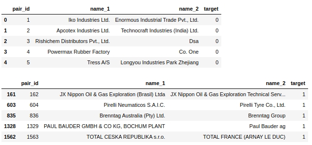
Some simple steps immediately suggest themselves: bring the text to one register, remove any stop words, such as 'ltd', delete countries and at the same time the names of geographical objects.
Actually, something like this can be solved in this task - you do some preprocessing, make sure that it works as it should, run the model, look at the quality and selectively analyze the objects on which the model is wrong. This is how I did my research. But in the article itself, the final solution is given and the quality of the algorithm after each preprocessing is not understood, at the end of the article we will conduct a final analysis. Otherwise, the article would be indescribable size :)
Let's make copies
To be honest, I don't know why I do this, but for some reason I always do it. I will do it this time too
The code
baseline_train = text_train.copy()
baseline_test = text_test.copy()
Convert all characters from text to lowercase
The code
# convert text to lowercase
columns = ['name_1','name_2']
for column in columns:
    lower_str(baseline_train,column)
for column in columns:
    lower_str(baseline_test,column)
Remove country names
It should be noted that the organizers of the competition are great fellows! Along with the assignment, they gave a laptop with a very simple baseline, in which was provided, including the code below.
The code
# drop any names of countries
countries = [country.name.lower() for country in pycountry.countries]
for country in tqdm(countries):
    baseline_train.replace(re.compile(country), "", inplace=True)
    baseline_test.replace(re.compile(country), "", inplace=True)
Remove signs and special characters
The code
# drop punctuation marks
baseline_train.replace(re.compile(r"\s+\(.*\)"), "", inplace=True)
baseline_test.replace(re.compile(r"\s+\(.*\)"), "", inplace=True)

baseline_train.replace(re.compile(r"[^\w\s]"), "", inplace=True)
baseline_test.replace(re.compile(r"[^\w\s]"), "", inplace=True)
Delete numbers
Removing the numbers from the text directly on the forehead, in the first attempt, greatly spoiled the quality of the model. I will give the code here, but in fact it was not used.
Also note that up to this point, we have performed the transformation directly on the columns that were given to us. Let's now create new columns for each preprocessing. There will be more columns, but if somewhere at some stage of preprocessing a failure occurs, it's okay, you don't need to do everything from the very beginning, because we will have columns from each stage of preprocessing.
Code that spoiled quality. You need to be more delicate
# # first: make dictionary of frequency every word
# list_words = baseline_train['name_1'].to_string(index=False).split() +\
#                 baseline_train['name_2'].to_string(index=False).split()
# freq_words = {}
# for w in list_words:
#     freq_words[w] = freq_words.get(w, 0) + 1

# # second: make data frame of frequency words
# df_freq = pd.DataFrame.from_dict(freq_words,orient='index').reset_index()
# df_freq.columns = ['word','frequency']
# df_freq_agg = df_freq.groupby(['word']).agg([sum]).reset_index()
# df_freq_agg = rename_agg_columns(id_client='word',data=df_freq_agg,rename='%s_%s')
# df_freq_agg = df_freq_agg.sort_values(by=['frequency_sum'], ascending=False)

# # third: make drop list of digits
# string = df_freq_agg['word'].to_string(index=False)
# digits = [int(digit) for digit in string.split() if digit.isdigit()]
# digits = set(digits)
# digits = list(digits)

# # drop the digits
# baseline_train['name_1_no_digits'] =\
#     baseline_train['name_1'].apply(
#     lambda x: ' '.join([word for word in x.split() if word not in (drop_list)]))
# baseline_train['name_2_no_digits'] =\
#     baseline_train['name_2'].apply(
#     lambda x: ' '.join([word for word in x.split() if word not in (drop_list)]))

# baseline_test['name_1_no_digits'] =\
#     baseline_test['name_1'].apply(
#     lambda x: ' '.join([word for word in x.split() if word not in (drop_list)]))
# baseline_test['name_2_no_digits'] =\
#     baseline_test['name_2'].apply(
#     lambda x: ' '.join([word for word in x.split() if word not in (drop_list)]))
Let's delete ... the first stopword list. Manually!
Now it is suggested to define and remove stop words from the word list in company names.
We have compiled the list based on manual review of the training sample. Logically, such a list should be compiled automatically using the following approaches:
- first, use the top 10 (20,50,100) common words.
- second, to use standard stop word libraries in different languages. For example, designations of organizational and legal forms of organizations in various languages (LLC, PJSC, CJSC, ltd, gmbh, inc, etc.)
- thirdly, it makes sense to compile a list of place names in different languages
We will come back to the first option for automatically compiling a list of top frequently encountered words, but for now we are looking at manual preprocessing.
The code
# drop some stop-words
drop_list = ["ltd.", "co.", "inc.", "b.v.", "s.c.r.l.", "gmbh", "pvt.",

             'retail','usa','asia','ceska republika','limited','tradig','llc','group',
             'international','plc','retail','tire','mills','chemical','korea','brasil',
             'holding','vietnam','tyre','venezuela','polska','americas','industrial','taiwan',
             'europe','america','north','czech republic','retailers','retails',

            'mexicana','corporation','corp','ltd','co','toronto','nederland','shanghai','gmb','pacific',
            'industries','industrias',

            'inc', 'ltda', '', '', '', '', '', '', '', '', 'ceska republika', 'ltda',
            'sibur', 'enterprises', 'electronics', 'products', 'distribution', 'logistics', 'development',
            'technologies', 'pvt', 'technologies', 'comercio', 'industria', 'trading', 'internacionais',
            'bank', 'sports',

            'express','east', 'west', 'south', 'north', 'factory', 'transportes', 'trade', 'banco',
            'management', 'engineering', 'investments', 'enterprise', 'city', 'national', 'express', 'tech',
            'auto', 'transporte', 'technology', 'and', 'central', 'american',

            'logistica','global','exportacao', 'ceska republika', 'vancouver', 'deutschland',

            'sro','rus','chemicals','private','distributors','tyres','industry','services','italia','beijing',

            '','company','the','und']

baseline_train['name_1_non_stop_words'] =\
    baseline_train['name_1'].apply(
    lambda x: ' '.join([word for word in x.split() if word not in (drop_list)]))
baseline_train['name_2_non_stop_words'] =\
    baseline_train['name_2'].apply(
    lambda x: ' '.join([word for word in x.split() if word not in (drop_list)]))

baseline_test['name_1_non_stop_words'] =\
    baseline_test['name_1'].apply(
    lambda x: ' '.join([word for word in x.split() if word not in (drop_list)]))
baseline_test['name_2_non_stop_words'] =\
    baseline_test['name_2'].apply(
    lambda x: ' '.join([word for word in x.split() if word not in (drop_list)]))
Let's selectively check that our stop words have actually been removed from the text.
The code
baseline_train[baseline_train.name_1_non_stop_words.str.contains("factory")].head(3)Table 4 "Selective check of the code to remove stop words"
Everything seems to work. Removed all stop words that are separated by a space. What we wanted. Moving on.
Let's transliterate the Russian text into the Latin alphabet
I use my self-written function and cyrtranslit library for this. It seems to work. Checked manually.
The code
# transliteration to latin
baseline_train['name_1_transliterated'] = transliterate(baseline_train['name_1_non_stop_words'])
baseline_train['name_2_transliterated'] = transliterate(baseline_train['name_2_non_stop_words'])
baseline_test['name_1_transliterated'] = transliterate(baseline_test['name_1_non_stop_words'])
baseline_test['name_2_transliterated'] = transliterate(baseline_test['name_2_non_stop_words'])
Let's look at a pair with id 353150. In it, the second column ("name_2") has the word "Michelin", after preprocessing the word is already written like this "mishlen" (see the column "name_2_transliterated"). Not entirely correct, but clearly better.
The code
pair_id = 353150
baseline_train[baseline_train['pair_id']==353150]
Table number 5 "Selective verification of the code for transliteration"

Let's start the automatic compilation of a list of the top 50 most common words & Drop it smart. First CHIT
A bit tricky title. Let's take a look at what we are going to do here.
First, we will combine the text from the first and second columns into one array and count for each unique word the number of times it occurs.
Second, let's pick the top 50 of these words. And it would seem that you can delete them, but no. These words may contain the names of holdings ('total', 'knauf', 'shell', ...), but this is very important information and it cannot be lost, since we will use it further. Therefore, we will go for a cheating (forbidden) trick. To begin with, on the basis of a careful, selective study of the training sample, we will compile a list of the names of frequently encountered holdings. The list will not be complete, otherwise it would not be fair at all :) Although, since we are not chasing a prize, why not. Then we will compare the array of the top 50 frequently occurring words with the list of holding names and remove from the list words that match the names of holdings.
The second stopword list is now complete. You can remove words from text.
But before that, I would like to insert a small remark regarding the cheating list of holding names. The fact that we have compiled a list of the names of holdings based on observations made our life much easier. But in fact, we could have compiled such a list in a different way. For example, you can take the ratings of the largest companies in the petrochemical, construction, automotive and other industries, combine them and take the names of holdings from there. But for the purposes of our research, we will restrict ourselves to a simple approach. This approach is prohibited within the competition! Moreover, the organizers of the competition, the work of candidates for the prize places are checked for prohibited techniques. Be careful!
The code
list_top_companies = ['arlanxeo', 'basf', 'bayer', 'bdp', 'bosch', 'brenntag', 'contitech',
                      'daewoo', 'dow', 'dupont', 'evonik', 'exxon', 'exxonmobil', 'freudenberg',
                      'goodyear', 'goter', 'henkel', 'hp', 'hyundai', 'isover', 'itochu', 'kia', 'knauf',
                      'kraton', 'kumho', 'lusocopla', 'michelin', 'paul bauder', 'pirelli', 'ravago',
                      'rehau', 'reliance', 'sabic', 'sanyo', 'shell', 'sherwinwilliams', 'sojitz',
                      'soprema', 'steico', 'strabag', 'sumitomo', 'synthomer', 'synthos',
                      'total', 'trelleborg', 'trinseo', 'yokohama']

# drop top 50 common words (NAME 1 & NAME 2) exept names of top companies

# first: make dictionary of frequency every word
list_words = baseline_train['name_1_transliterated'].to_string(index=False).split() +\
                baseline_train['name_2_transliterated'].to_string(index=False).split()
freq_words = {}
for w in list_words:
    freq_words[w] = freq_words.get(w, 0) + 1

# # second: make data frame
df_freq = pd.DataFrame.from_dict(freq_words,orient='index').reset_index()
df_freq.columns = ['word','frequency']
df_freq_agg = df_freq.groupby(['word']).agg([sum]).reset_index()
df_freq_agg = rename_agg_columns(id_client='word',data=df_freq_agg,rename='%s_%s')
df_freq_agg = df_freq_agg.sort_values(by=['frequency_sum'], ascending=False)
drop_list = list(set(df_freq_agg[0:50]['word'].to_string(index=False).split()) - set(list_top_companies))

# # check list of top 50 common words
# print (drop_list)

# drop the top 50 words
baseline_train['name_1_finish'] =\
    baseline_train['name_1_transliterated'].apply(
    lambda x: ' '.join([word for word in x.split() if word not in (drop_list)]))
baseline_train['name_2_finish'] =\
    baseline_train['name_2_transliterated'].apply(
    lambda x: ' '.join([word for word in x.split() if word not in (drop_list)]))

baseline_test['name_1_finish'] =\
    baseline_test['name_1_transliterated'].apply(
    lambda x: ' '.join([word for word in x.split() if word not in (drop_list)]))
baseline_test['name_2_finish'] =\
    baseline_test['name_2_transliterated'].apply(
    lambda x: ' '.join([word for word in x.split() if word not in (drop_list)]))
This is where we are done with data preprocessing. Let's start generating new features and visually assessing them for the ability to separate objects by 0 or 1.
Feature generation and analysis
Let's calculate the Levenshtein distance
Let's use the strsimpy library and in each pair (after all the preprocessing) we will calculate the Levenshtein distance from the company name from the first column to the company name in the second column.
The code
# create feature with LEVENSTAIN DISTANCE
levenshtein = Levenshtein()
column_1 = 'name_1_finish'
column_2 = 'name_2_finish'

baseline_train["levenstein"] = baseline_train.progress_apply(
    lambda r: levenshtein.distance(r[column_1], r[column_2]), axis=1)
baseline_test["levenstein"] = baseline_test.progress_apply(
    lambda r: levenshtein.distance(r[column_1], r[column_2]), axis=1)
Let's calculate the normalized Levenshtein distance
Everything is the same as above, only we will count the normalized distance.
Spoiler header
# create feature with NORMALIZATION LEVENSTAIN DISTANCE
normalized_levenshtein = NormalizedLevenshtein()
column_1 = 'name_1_finish'
column_2 = 'name_2_finish'

baseline_train["norm_levenstein"] = baseline_train.progress_apply(
    lambda r: normalized_levenshtein.distance(r[column_1], r[column_2]),axis=1)
baseline_test["norm_levenstein"] = baseline_test.progress_apply(
    lambda r: normalized_levenshtein.distance(r[column_1], r[column_2]),axis=1)
We counted, and now we visualize
Visualizing features
Let's look at the distribution of the trait 'levenstein'
The code
data = baseline_train
analyse = 'levenstein'
size = (12,2)
dd = data_statistics(data,analyse,title_print='no')
hist_fz(data,dd,analyse,size)
boxplot(data,analyse,size)
Graphs # 1 "Histogram and box with a mustache for assessing the significance of a feature"
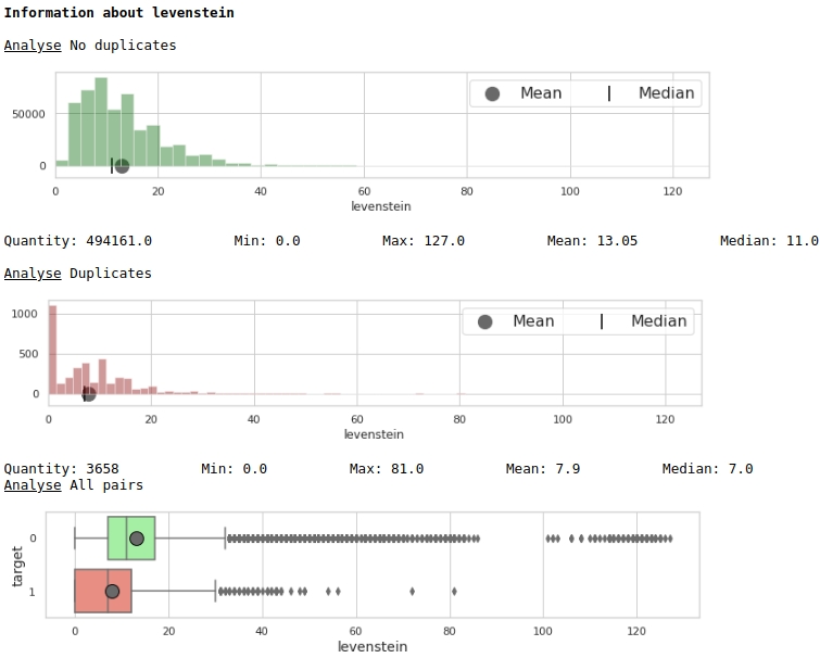
At first glance, a metric can mark up data. Obviously not very good, but it can be used.
Let's look at the distribution of the trait 'norm_levenstein'
Spoiler header
data = baseline_train
analyse = 'norm_levenstein'
size = (14,2)
dd = data_statistics(data,analyse,title_print='no')
hist_fz(data,dd,analyse,size)
boxplot(data,analyse,size)
Graphs №2 "Histogram and box with a mustache for assessing the significance of the sign"

Already better. Now, let's take a look at how the two combined features will divide the space into objects 0 and 1.
The code
data = baseline_train
analyse1 = 'levenstein'
analyse2 = 'norm_levenstein'
size = (14,6)
two_features(data,analyse1,analyse2,size)
Graph # 3 "Scatter diagram"
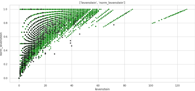
Very good markup is obtained. So it's not for nothing that we pre-processed the data so much :)
Everyone understands that horizontally - the values of the metric "levenstein", and vertically - the values of the metric "norm_levenstein", and the green and black points are objects 0 and 1. We move on.
Let's compare words in the text for each pair and generate a large bunch of features
Below we will compare the words in company names. Let's create the following features:
- a list of words that are duplicated in columns # 1 and # 2 of each pair
- a list of words that are NOT duplicated
Based on these lists of words, we will create the features that we will feed into the trained model:
- number of duplicate words
- number of NOT duplicated words
- sum of characters, duplicate words
- sum of characters, NOT duplicate words
- average length of duplicate words
- average length of NOT duplicated words
- the ratio of the number of duplicates to the number of NOT duplicates
The code here is probably not very friendly, since, again, it was written in haste. But it works, but it will go for a quick research.
The code
# make some information about duplicates and differences for TRAIN
column_1 = 'name_1_finish'
column_2 = 'name_2_finish'

duplicates = []
difference = []

for i in range(baseline_train.shape[0]):
    list1 = list(baseline_train[i:i+1][column_1])
    str1 = ''.join(list1).split()
    list2 = list(baseline_train[i:i+1][column_2])
    str2 = ''.join(list2).split()

    duplicates.append(list(set(str1) & set(str2)))
    difference.append(list(set(str1).symmetric_difference(set(str2))))

# continue make information about duplicates
duplicate_count,duplicate_sum = compair_metrics(duplicates)
dif_count,dif_sum = compair_metrics(difference)

# create features have information about duplicates and differences for TRAIN
baseline_train['duplicate'] = duplicates
baseline_train['difference'] = difference

baseline_train['duplicate_count'] = duplicate_count
baseline_train['duplicate_sum'] = duplicate_sum
baseline_train['duplicate_mean'] = baseline_train['duplicate_sum'] / baseline_train['duplicate_count']
baseline_train['duplicate_mean'] = baseline_train['duplicate_mean'].fillna(0)

baseline_train['dif_count'] = dif_count
baseline_train['dif_sum'] = dif_sum
baseline_train['dif_mean'] = baseline_train['dif_sum'] / baseline_train['dif_count']
baseline_train['dif_mean'] = baseline_train['dif_mean'].fillna(0)

baseline_train['ratio_duplicate/dif_count'] = baseline_train['duplicate_count'] / baseline_train['dif_count']

# make some information about duplicates and differences for TEST
column_1 = 'name_1_finish'
column_2 = 'name_2_finish'

duplicates = []
difference = []

for i in range(baseline_test.shape[0]):
    list1 = list(baseline_test[i:i+1][column_1])
    str1 = ''.join(list1).split()
    list2 = list(baseline_test[i:i+1][column_2])
    str2 = ''.join(list2).split()

    duplicates.append(list(set(str1) & set(str2)))
    difference.append(list(set(str1).symmetric_difference(set(str2))))

# continue make information about duplicates
duplicate_count,duplicate_sum = compair_metrics(duplicates)
dif_count,dif_sum = compair_metrics(difference)

# create features have information about duplicates and differences for TEST
baseline_test['duplicate'] = duplicates
baseline_test['difference'] = difference

baseline_test['duplicate_count'] = duplicate_count
baseline_test['duplicate_sum'] = duplicate_sum
baseline_test['duplicate_mean'] = baseline_test['duplicate_sum'] / baseline_test['duplicate_count']
baseline_test['duplicate_mean'] = baseline_test['duplicate_mean'].fillna(0)

baseline_test['dif_count'] = dif_count
baseline_test['dif_sum'] = dif_sum
baseline_test['dif_mean'] = baseline_test['dif_sum'] / baseline_test['dif_count']
baseline_test['dif_mean'] = baseline_test['dif_mean'].fillna(0)

baseline_test['ratio_duplicate/dif_count'] = baseline_test['duplicate_count'] / baseline_test['dif_count']
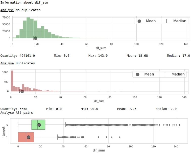
We visualize some of the signs.
The code
data = baseline_train
analyse = 'dif_sum'
size = (14,2)
dd = data_statistics(data,analyse,title_print='no')
hist_fz(data,dd,analyse,size)
boxplot(data,analyse,size)
Graphs No. 4 "Histogram and a box with a mustache for assessing the significance of the sign"
The code
data = baseline_train
analyse1 = 'duplicate_mean'
analyse2 = 'dif_mean'
size = (14,6)
two_features(data,analyse1,analyse2,size)
Graph №5 "Scatter diagram"
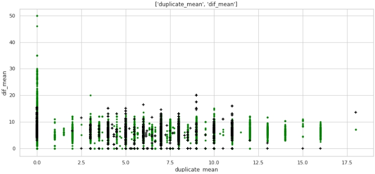
What no, but the markup. Note that a lot of companies with a target label of 1 have zero duplicates in the text, and also a lot of companies with duplicates in their names, on average more than 12 words, belong to companies with a target label of 0.
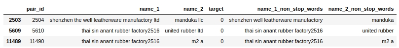
Let's take a look at the tabular data, prepare a query for In the first case: there are zero duplicates in the name of the companies, but the companies are the same.
The code
baseline_train[
    baseline_train['duplicate_mean']==0][
    baseline_train['target']==1].drop(
        ['duplicate', 'difference',
        'name_1_non_stop_words',
        'name_2_non_stop_words', 'name_1_transliterated',
        'name_2_transliterated'],axis=1)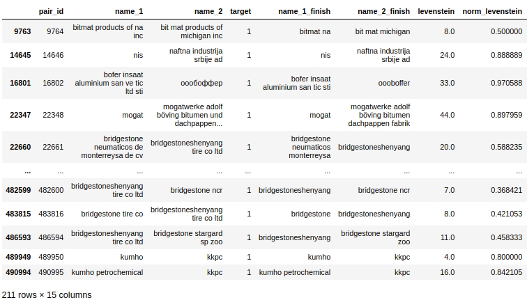
Obviously there is a system error in our processing. We did not take into account that words can be spelled not only with errors, but also simply together or, on the contrary, separately where this is not required. For example, pair # 9764. In the first column 'bitmat' in the second 'bit mat' and now this is not a double, but the company is the same. Or another example, pair # 482600 'bridgestoneshenyang' and 'bridgestone'.
What could be done. The first thing that occurred to me was to compare not directly head-on, but using the Levenshtein metric. But here, too, an ambush awaits us: the distance between 'bridgestoneshenyang' and 'bridgestone' will not be small. Perhaps lemmatization will come to the rescue, but again it is not immediately clear how the names of companies can be lemmatized. Or you can use the Tamimoto coefficient, but let's leave this moment for more experienced comrades and move on.
Let's compare words from the text with words from the names of the top 50 holding brands in the petrochemical, construction and other industries. Let's get the second big pile of features. Second CHIT
In fact, there are two violations of the rules for participating in the competition:
- -, , «duplicate_name_company»
- -, . , .
Both techniques are prohibited by the competition rules. You can bypass the ban. To do this, you need to compile a list of holding names not manually based on a selective view of the training sample, but automatically - from external sources. But then, firstly, the list of holdings will turn out to be large and the comparison of words proposed in the work will take very, well, just a lot of time, and secondly, this list still needs to be compiled :) Therefore, for the purposes of simplicity of research, we will check how much the quality of the model will improve with these signs. Running ahead - the quality is growing just amazing!
With the first method, everything seems to be clear, but the second approach requires explanations.
So, let's determine the Levenshtein distance from each word in each line of the first column with the company name to each word from the list of top petrochemical companies (and not only).
If the ratio of the Levenshtein distance to the word length is less than or equal to 0.4, then we determine the ratio of the Levenshtein distance to the selected word from the list of top companies to each word from the second column - the name of the second company.
If the second coefficient (the ratio of distance to word length from the list of top companies) turns out to be below or equal to 0.4, then we fix the following values in the table:
- Levenshtein distance from a word from the list of No. 1 companies to a word in the list of top companies
- Levenshtein distance from a word from the list of No. 2 companies to a word in the list of top companies
- length of a word from list # 1
- length of a word from list # 2
- word length from the list of top companies
- the ratio of the length of a word from the list # 1 to the distance
- the ratio of the length of a word from the list No. 2 to the distance
There can be more than one match in one line, let's choose the minimum of them (aggregation function).
I would like to draw your attention once again to the fact that the proposed method for generating features is quite resource-intensive and in case of obtaining a list from an external source, a change in the code for compiling metrics will be required.
The code
# create information about duplicate name of petrochemical companies from top list
list_top_companies = list_top_companies

dp_train = []
for i in list(baseline_train['duplicate']):
    dp_train.append(''.join(list(set(i) & set(list_top_companies))))

dp_test = []
for i in list(baseline_test['duplicate']):
    dp_test.append(''.join(list(set(i) & set(list_top_companies))))

baseline_train['duplicate_name_company'] = dp_train
baseline_test['duplicate_name_company'] = dp_test

# replace name duplicate to number
baseline_train['duplicate_name_company'] =\
    baseline_train['duplicate_name_company'].replace('',0,regex=True)
baseline_train.loc[baseline_train['duplicate_name_company'] != 0, 'duplicate_name_company'] = 1

baseline_test['duplicate_name_company'] =\
    baseline_test['duplicate_name_company'].replace('',0,regex=True)
baseline_test.loc[baseline_test['duplicate_name_company'] != 0, 'duplicate_name_company'] = 1

# create some important feature about similar words in the data and names of top companies for TRAIN
# (levenstein distance, length of word, ratio distance to length)
baseline_train = dist_name_to_top_list_make(baseline_train,
                      'name_1_finish','name_2_finish',list_top_companies)

# create some important feature about similar words in the data and names of top companies for TEST
# (levenstein distance, length of word, ratio distance to length)
baseline_test = dist_name_to_top_list_make(baseline_test,
                      'name_1_finish','name_2_finish',list_top_companies)
Let's look at the usefulness of features through the prism of charts
The code
data = baseline_train
analyse = 'levenstein_dist_w1_top_w_min'
size = (14,2)
dd = data_statistics(data,analyse,title_print='no')
hist_fz(data,dd,analyse,size)
boxplot(data,analyse,size)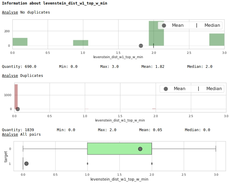
Very good.
Preparing data for submission to the model
We have got a large table and we do not need all the data for analysis. Let's look at the names of the table columns.
The code
baseline_train.columns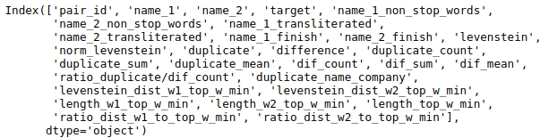
Let's select those columns that we will analyze.
Let's fix the seed for the reproducibility of the result.
The code
# fix some parameters
features = ['levenstein','norm_levenstein',

            'duplicate_count','duplicate_sum','duplicate_mean',
            'dif_count','dif_sum','dif_mean','ratio_duplicate/dif_count',

            'duplicate_name_company',

           'levenstein_dist_w1_top_w_min', 'levenstein_dist_w2_top_w_min',
       'length_w1_top_w_min', 'length_w2_top_w_min', 'length_top_w_min',
       'ratio_dist_w1_to_top_w_min', 'ratio_dist_w2_to_top_w_min'
            ]
seed = 42
Before finally training the model on all available data and sending the solution for verification, it makes sense to test the model. To do this, we split the training sample into conditionally training and conditionally test. We will measure the quality on it and if it suits us, we will send the solution to the competition.
The code
# provides train/test indices to split data in train/test sets
split = StratifiedShuffleSplit(n_splits=1, train_size=0.8, random_state=seed)

tridx, cvidx = list(split.split(baseline_train[features],
                                baseline_train["target"]))[0]

print ('Split baseline data train',baseline_train.shape[0])
print (' - new train data:',tridx.shape[0])
print (' - new test data:',cvidx.shape[0])
Setting up and training the model
We will use a decision tree from the Light GBM library as a model.
It makes no sense to wind up the parameters too much. We look at the code.
The code
# learning Light GBM Classificier
seed = 50
params = {'n_estimators': 1,
          'objective': 'binary',
          'max_depth': 40,
          'min_child_samples': 5,
          'learning_rate': 1,
#           'reg_lambda': 0.75,
#           'subsample': 0.75,
#           'colsample_bytree': 0.4,
#           'min_split_gain': 0.02,
#           'min_child_weight': 40,
          'random_state': seed}


model = lgb.LGBMClassifier(**params)
model.fit(baseline_train.iloc[tridx][features].values,
          baseline_train.iloc[tridx]["target"].values)
The model was tuned and trained. Now let's look at the results.
The code
# make predict proba and predict target
probability_level = 0.99
X = baseline_train
tridx = tridx
cvidx = cvidx
model = model

X_tr, X_cv = contingency_table(X,features,probability_level,tridx,cvidx,model)

train_matrix_confusion = matrix_confusion(X_tr)
cv_matrix_confusion = matrix_confusion(X_cv)

report_score(train_matrix_confusion,
             cv_matrix_confusion,
             baseline_train,
             tridx,cvidx,
             X_tr,X_cv)
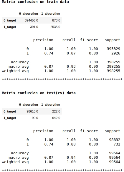
Note that we are using the f1 quality metric as the model score. This means that it makes sense to regulate the level of probability of assigning an object to class 1 or 0. We have chosen the level of 0.99, that is, if the probability is equal to or higher than 0.99, the object will be assigned to class 1, below 0.99 - to class 0. This is an important point - you can significantly improve the speed such a tricky simple trick.
The quality seems to be not bad. On a conditionally test sample, the algorithm made mistakes when defining 222 objects of class 0 and on 90 objects belonging to class 0 it made a mistake and assigned them to class 1 (see Matrix confusion on test (cv) data).
Let's see which signs were the most important and which were not.
The code
start = 0
stop = 50
size = (12,6)

tg = table_gain_coef(model,features,start,stop)
gain_hist(tg,size,start,stop)
display(tg)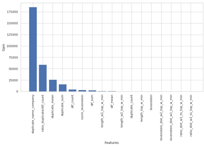
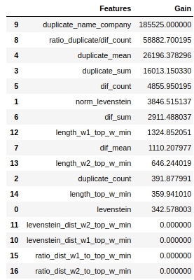
Note that we used the 'gain' parameter, not the 'split' parameter to assess the significance of the features. This is important because, in a very simplified version, the first parameter means the contribution of the feature to the decrease in entropy, and the second indicates how many times the feature has been used to mark the space.
At first glance, the feature that we have been doing for a very long time, "levenstein_dist_w1_top_w_min", turned out to be not informative at all - its contribution is 0. But this is only at first glance. It is simply almost completely duplicated in meaning with the "duplicate_name_company" attribute. If you delete "duplicate_name_company" and leave "levenstein_dist_w1_top_w_min", then the second attribute will take the place of the first one and the quality will not change. Checked!
In general, such a sign is a handy thing, especially when you have hundreds of features and a model with a bunch of bells and whistles and 5000 iterations. You can remove features in batches and watch the quality grow from this not cunning action. In our case, removal of features will not affect the quality.
Let's take a look at the mate table. First of all, let's look at the objects "False Positive", that is, those that our algorithm determined to be the same and assigned them to class 1, but in fact they belong to class 0.
The code
X_cv[X_cv['False_Positive']==1][0:50].drop(['name_1_non_stop_words',
       'name_2_non_stop_words', 'name_1_transliterated',
       'name_2_transliterated', 'duplicate', 'difference',
       'levenstein',
       'levenstein_dist_w1_top_w_min', 'levenstein_dist_w2_top_w_min',
       'length_w1_top_w_min', 'length_w2_top_w_min', 'length_top_w_min',
       'ratio_dist_w1_to_top_w_min', 'ratio_dist_w2_to_top_w_min',
       'True_Positive','True_Negative','False_Negative'],axis=1)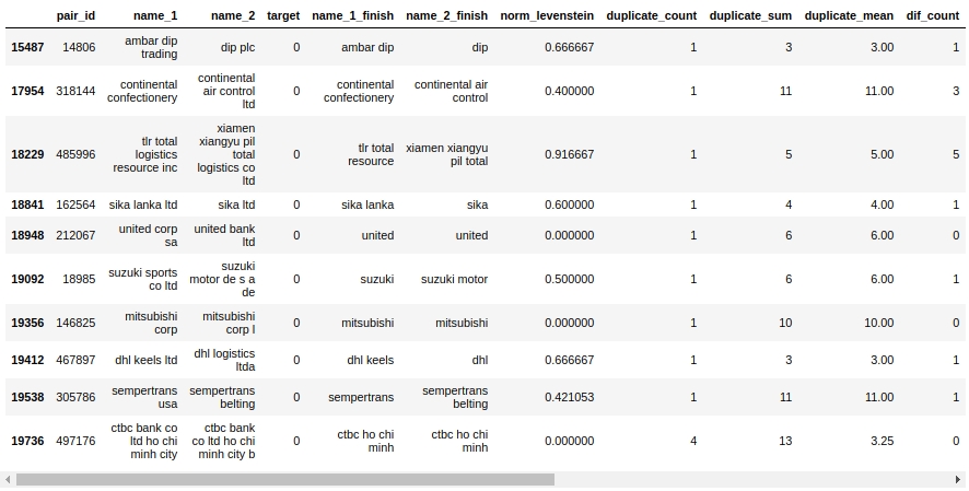
Yeah. Here, a person will not immediately determine 0 or 1. For example, pair # 146825 "mitsubishi corp" and "mitsubishi corp l". The eyes say it's the same thing, but the sample says it's different companies. Whom to believe?
Let's just say that you could squeeze out right away - we squeezed out. We will leave the rest of the work to experienced comrades :)
Let's upload the data to the organizer's website and find out the assessment of the quality of the work.
Results of the competition
The code
model = lgb.LGBMClassifier(**params)
model.fit(baseline_train[features].values,
          baseline_train["target"].values)

sample_sub = pd.read_csv('sample_submission.csv', index_col="pair_id")

sample_sub['is_duplicate'] = (model.predict_proba(
    baseline_test[features].values)[:, 1] > probability_level).astype(np.int)

sample_sub.to_csv('baseline_submission.csv')
So, our fast, taking into account the prohibited method: 0.5999
Without it, the quality was somewhere between 0.3 and 0.4. We need to restart the model for accuracy, but I'm a little too lazy :)
Let's better summarize the experience gained.
First, as you can see, we have got quite reproducible code and a fairly adequate file structure. Due to my little experience, at one time I got a lot of bumps precisely because I was filling out the work in a hurry, just to get some more or less pleasant speed. As a result, the file turned out to be such that after a week it was already scary to open it - nothing is so clear. Therefore, my message is to immediately write the code and make the file readable, so that in a year you can return to the data, look at the structure first, understand what steps were taken and then so that each step can be easily disassembled. Of course, if you are a beginner, then on the first try the file will not be beautiful, the code will break, there will be crutches, but if you periodically rewrite the code during the research process,then by 5-7 rewriting times you yourself will be surprised at how much cleaner the code is and maybe even find errors and improve the speed. Don't forget about the functions, it makes the file very easy to read.
Secondly, after each processing of the data, check if everything went as intended. To do this, you need to be able to filter tables in pandas. There is a lot of filtering in this work, use it for health :)
Third, always, downright always, in classification tasks, form both a table and a conjugation matrix. From the table, you can easily find on which objects the algorithm is wrong. To begin with, try to notice those errors that are called system errors, they require less work to fix, and give more results. Then, as you sort out the system errors, go to special cases. By the error matrix, you will see where the algorithm makes more mistakes: on class 0 or 1. From here you will dig errors. For example, I noticed that my tree defines classes 1 well, but makes a lot of mistakes on class 0, that is, the tree often "says" that this object is of class 1, when in fact it is 0. I assumed that it might be associated with the level of probability of classifying an object as 0 or 1. My level was fixed at 0.9.The increase in the level of probability of assigning an object to class 1 to 0.99 made the selection of objects of class 1 tougher and voila - our speed has given a significant increase.
Once again, I will note that the purpose of participating in the competition was not to win a prize, but to gain experience. Considering that before the start of the competition, I had no idea how to work with texts in machine learning, and as a result, in a few days I got a simple, but still working model, then we can say the goal has been achieved. Also, for any novice samurai in the world of data science, I think it is important to gain experience, not a prize, or rather, experience is the prize. Therefore, do not be afraid to participate in competitions, go for it, everyone is a beaver!
At the time of publication of the article, the competition is not over yet. Based on the results of the completion of the competition, in the comments to the article, I will write about the maximum fair speed, about the approaches and features that improve the quality of the model.
And you are a dear reader, if you have ideas on how to increase the speed right now, write in the comments. Do a good deed :)
Sources of information, auxiliary materials
- "Github with Data and Jupyter Notebook"
- "SIBUR CHALLENGE 2020 Competition Platform"
- "Site of the organizer of the competition SIBUR CHALLENGE 2020"
- "Good article on Habré" Fundamentals of Natural Language Processing for Text ""
- "Another good article on Habré" Fuzzy string comparison: understand me if you can ""
- "Publication from the APNI magazine"
- "An article about Tanimoto coefficient" String similarity "not used here"