LightGBM extends the Gradient Boosting algorithm by adding a type of automatic object selection as well as focusing on examples of boosting with large gradients. This can lead to dramatic acceleration of learning and better predictive performance. Thus, LightGBM has become the de facto algorithm for machine learning competitions when working with tabular data for regression and classification predictive modeling problems. This tutorial will show you how to design Light Gradient Boosted Machine Ensembles for Classification and Regression. After completing this tutorial, you will know:
- The Light Gradient Boosted Machine (LightGBM) is an efficient open source implementation of the stochastic gradient boosting ensemble.
- How to develop LightGBM ensembles for classification and regression using scikit-learn API.
- LightGBM .

- LightBLM.
- Scikit-Learn API LightGBM.
— LightGBM .
— LightGBM . - LightGBM.
— .
— .
— .
— .
LightBLM
Gradient boosting belongs to a class of ensemble machine learning algorithms that can be used for classification problems or predictive regression modeling.
Ensembles are built based on decision tree models. The trees are added one at a time to the ensemble and trained to correct the prediction errors made by the previous models. This is a type of ensemble machine learning model called boosting.
The models are trained using any arbitrary differentiable loss function and a gradient descent optimization algorithm. This gives the method its name "gradient boosting" because the loss gradient is minimized as the model is trained, like a neural network. For more information on gradient boosting, see the tutorial:"A gentle introduction to the ML gradient boosting algorithm . "
LightGBM is an open source implementation of gradient boosting designed to be efficient and even possibly more efficient than other implementations.
As such, LightGBM is an open source project, software library, and machine learning algorithm. That is, the project is very similar to the Extreme Gradient Boosting or XGBoost technique .
LightGBM has been described by Golin, K., et al. For more information, see a 2017 article entitled "LightGBM: A Highly Efficient Gradient Boosting Decision Tree . " The implementation introduces two key ideas: GOSS and EFB.
Gradient One-Way Sampling (GOSS) is a modification of Gradient Boosting that focuses on those tutorials that result in a larger gradient, which in turn speeds up learning and reduces the computational complexity of the method.
With GOSS, we exclude a significant portion of the data instances with small gradients and use only the rest of the data instances to estimate the gain in information. We argue that since data instances with large gradients play a more important role in computing the information gain, GOSS can obtain a fairly accurate estimate of the information gain with a much smaller data size.
Exclusive Feature Bundling, or EFB, is an approach of combining sparse (mostly null) mutually exclusive features, such as categorical input variables encoded with a unitary encoding. Thus, it is a type of automatic feature selection.
... we package mutually exclusive features (that is, they rarely take non-zero values at the same time) to reduce the number of features.
Together, these two changes can speed up the training time of the algorithm by up to 20 times. Thus, LightGBM can be thought of as Gradient Boosted Decision Trees (GBDTs) with the addition of GOSS and EFB.
We call our new GBDT implementation GOSS and EFB LightGBM. Our experiments on several publicly available datasets show that LightGBM accelerates the learning process of a conventional GBDT by more than 20 times, achieving almost the same accuracy.
Scikit-Learn API for LightGBM
LightGBM can be installed as a stand-alone library and the LightGBM model can be developed using the scikit-learn API.
The first step is to install the LightGBM library. On most platforms it can be done using the pip package manager; eg:
sudo pip install lightgbmYou can check the installation and version like this:
# check lightgbm version
import lightgbm
print(lightgbm.__version__)
The script will display the version of installed LightGBM. Your version should be the same or higher. If not, update LightGBM. If you need specific instructions for your development environment, refer to the LightGBM Installation Guide .
The LightGBM library has its own API, although we are using a method through scikit-learn wrapper classes: LGBMRegressor and LGBMClassifier . This will allow you to apply the entire set of tools from the scikit-learn machine learning library for data preparation and model evaluation.
Both models work in the same way and use the same arguments to influence how decision trees are created and added to the ensemble. The model uses randomness. This means that every time the algorithm runs on the same data, it creates a slightly different model.
When using machine learning algorithms with a stochastic learning algorithm, it is recommended to evaluate them by averaging their performance over several runs or repetitions of cross-validation. When fitting the final model, it may be desirable to either increase the number of trees until the variance of the model decreases with repeated estimates, or to train several final models and average their predictions. Let's take a look at designing a LightGBM ensemble for both classification and regression.
LightGBM ensemble for classification
In this section, we'll look at using LightGBM for a classification task. First, we can use the make_classification () function to create a synthetic binary classification problem with 1000 examples and 20 input features. See the whole example below.
# test classification dataset
from sklearn.datasets import make_classification
# define dataset
X, y = make_classification(n_samples=1000, n_features=20, n_informative=15, n_redundant=5, random_state=7)
# summarize the dataset
Running the example creates a dataset and summarizes the shape of the input and output components.
(1000, 20) (1000,)We can then evaluate the LightGBM algorithm on this dataset. We will evaluate the model using a repeated stratified k-fold cross-validation with three repetitions and a k of 10. We will report the mean and standard deviation of the model accuracy over all repetitions and folds.
# evaluate lightgbm algorithm for classification
from numpy import mean
from numpy import std
from sklearn.datasets import make_classification
from sklearn.model_selection import cross_val_score
from sklearn.model_selection import RepeatedStratifiedKFold
from lightgbm import LGBMClassifier
# define dataset
X, y = make_classification(n_samples=1000, n_features=20, n_informative=15, n_redundant=5, random_state=7)
# define the model
model = LGBMClassifier()
# evaluate the model
cv = RepeatedStratifiedKFold(n_splits=10, n_repeats=3, random_state=1)
n_scores = cross_val_score(model, X, y, scoring='accuracy', cv=cv, n_jobs=-1)
# report performance
print('Accuracy: %.3f (%.3f)' % (mean(n_scores), std(n_scores)))
Running the example shows the accuracy of the mean and standard deviation of the model.
Note : Your results may differ due to the stochastic nature of the algorithm or estimation procedure, or differences in numerical precision. Try the example several times and compare the average result.
In this case, we can see that the LightGBM ensemble with default hyperparameters achieves a classification accuracy of around 92.5% on this test dataset.
Accuracy: 0.925 (0.031)We can also use the LightGBM model as the final model and make predictions for classification. First, the LightGBM ensemble fits all available data, and second, you can call the predict () function to make predictions on the new data. The example below demonstrates this on our binary classification dataset.
# make predictions using lightgbm for classification
from sklearn.datasets import make_classification
from lightgbm import LGBMClassifier
# define dataset
X, y = make_classification(n_samples=1000, n_features=20, n_informative=15, n_redundant=5, random_state=7)
# define the model
model = LGBMClassifier()
# fit the model on the whole dataset
model.fit(X, y)
# make a single prediction
row = [0.2929949,-4.21223056,-1.288332,-2.17849815,-0.64527665,2.58097719,0.28422388,-7.1827928,-1.91211104,2.73729512,0.81395695,3.96973717,-2.66939799,3.34692332,4.19791821,0.99990998,-0.30201875,-4.43170633,-2.82646737,0.44916808]
yhat = model.predict([row])
print('Predicted Class: %d' % yhat[0])
Running the example trains a LightGBM ensemble model for the entire dataset and then uses it to predict a new row of data, as it would if the model were used in an application.
Predicted Class: 1Now that we are familiar with using LightGBM for classification, let's take a look at the regression API.
LightGBM Ensemble for Regression
In this section, we will look at using LightGBM for a regression problem. First, we can use the make_regression () function
to create a synthetic regression problem with 1000 examples and 20 input features. See the whole example below.
# test regression dataset
from sklearn.datasets import make_regression
# define dataset
X, y = make_regression(n_samples=1000, n_features=20, n_informative=15, noise=0.1, random_state=7)
# summarize the dataset
print(X.shape, y.shape)
Running the example creates a dataset and summarizes the input and output components.
(1000, 20) (1000,)Second, we can evaluate the LightGBM algorithm on this dataset.
As in the last section, we will evaluate the model by repeated k-fold cross-validation with three replicates and k equal to 10. We will report the mean absolute error (MAE) of the model across all replicates and cross-validation groups. The scikit-learn library makes the MAE negative so that it is maximized rather than minimized. This means that large negative MAEs are better and the ideal model has an MAE of 0. A complete example is shown below.
# evaluate lightgbm ensemble for regression
from numpy import mean
from numpy import std
from sklearn.datasets import make_regression
from sklearn.model_selection import cross_val_score
from sklearn.model_selection import RepeatedKFold
from lightgbm import LGBMRegressor
# define dataset
X, y = make_regression(n_samples=1000, n_features=20, n_informative=15, noise=0.1, random_state=7)
# define the model
model = LGBMRegressor()
# evaluate the model
cv = RepeatedKFold(n_splits=10, n_repeats=3, random_state=1)
n_scores = cross_val_score(model, X, y, scoring='neg_mean_absolute_error', cv=cv, n_jobs=-1, error_score='raise')
# report performance
print('MAE: %.3f (%.3f)' % (mean(n_scores), std(n_scores)))
Running the example reports the mean and standard deviation of the model.
Note : Your results may vary due to the stochastic nature of the algorithm or estimation procedure, or differences in numerical precision. Consider running the example multiple times and comparing the average. In this case, we see that the LightGBM ensemble with default hyperparameters reaches an MAE of around 60.
MAE: -60.004 (2.887)We can also use the LightGBM model as the final model and make predictions for the regression. First, the LightGBM ensemble is trained on all available data, then predict () can be called to predict new data. The example below demonstrates this on our regression dataset.
# gradient lightgbm for making predictions for regression
from sklearn.datasets import make_regression
from lightgbm import LGBMRegressor
# define dataset
X, y = make_regression(n_samples=1000, n_features=20, n_informative=15, noise=0.1, random_state=7)
# define the model
model = LGBMRegressor()
# fit the model on the whole dataset
model.fit(X, y)
# make a single prediction
row = [0.20543991,-0.97049844,-0.81403429,-0.23842689,-0.60704084,-0.48541492,0.53113006,2.01834338,-0.90745243,-1.85859731,-1.02334791,-0.6877744,0.60984819,-0.70630121,-1.29161497,1.32385441,1.42150747,1.26567231,2.56569098,-0.11154792]
yhat = model.predict([row])
print('Prediction: %d' % yhat[0])
Running the example trains the LightGBM ensemble model on the entire dataset and then uses it to predict a new row of data, as it would if using the model in an application.
Prediction: 52Now that we are familiar with using the scikit-learn API to evaluate and apply LightGBM ensembles, let's take a look at setting up the model.
LightGBM Hyperparameters
In this section, we'll take a closer look at some of the hyperparameters that are important to the LightGBM ensemble and their impact on model performance. LightGBM has a lot of hyperparameters to look at, here we look at the number of trees and their depth, the learning rate and the type of boost. For general tips on tweaking LightGBM hyperparameters, see the documentation: Tuning LightGBM Parameters .
Examining the number of trees
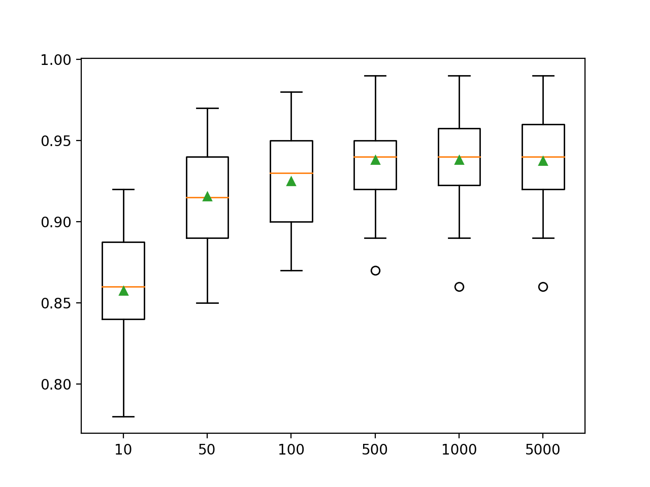
An important hyperparameter for the LightGBM ensemble algorithm is the number of decision trees used in the ensemble. Recall that decision trees are added to the model sequentially in an attempt to correct and improve the predictions made by previous trees. The rule often works: more trees is better. The number of trees can be specified using the n_estimators argument, which defaults to 100. The example below examines the effect of the number of trees, from 10 to 5000.
# explore lightgbm number of trees effect on performance
from numpy import mean
from numpy import std
from sklearn.datasets import make_classification
from sklearn.model_selection import cross_val_score
from sklearn.model_selection import RepeatedStratifiedKFold
from lightgbm import LGBMClassifier
from matplotlib import pyplot

# get the dataset
def get_dataset():
X, y = make_classification(n_samples=1000, n_features=20, n_informative=15, n_redundant=5, random_state=7)
return X, y

# get a list of models to evaluate
def get_models():
models = dict()
trees = [10, 50, 100, 500, 1000, 5000]
for n in trees:
models[str(n)] = LGBMClassifier(n_estimators=n)
return models

# evaluate a give model using cross-validation
def evaluate_model(model):
cv = RepeatedStratifiedKFold(n_splits=10, n_repeats=3, random_state=1)
scores = cross_val_score(model, X, y, scoring='accuracy', cv=cv, n_jobs=-1)
return scores

# define dataset
X, y = get_dataset()
# get the models to evaluate
models = get_models()
# evaluate the models and store results
results, names = list(), list()
for name, model in models.items():
scores = evaluate_model(model)
results.append(scores)
names.append(name)
print('>%s %.3f (%.3f)' % (name, mean(scores), std(scores)))
# plot model performance for comparison
pyplot.boxplot(results, labels=names, showmeans=True)
pyplot.show()
Running the example first displays the average precision for each number of decision trees.
Note : Your results may differ due to the stochastic nature of the algorithm or estimation procedure, or differences in numerical precision. Consider running the example multiple times and comparing the average.
Here we see that performance improves for this dataset to about 500 trees, after which it seems to level out.
>10 0.857 (0.033)
>50 0.916 (0.032)
>100 0.925 (0.031)
>500 0.938 (0.026)
>1000 0.938 (0.028)
>5000 0.937 (0.028)
A box and whisker plot is created to distribute the accuracy scores for each configured number of trees. There is a general trend towards an increase in model performance and ensemble size.
Examining the depth of a tree
Changing the depth of each tree added to the ensemble is another important hyperparameter for gradient boosting. The depth of the tree determines how much each tree specializes in the training dataset: how general or trained it can be. Trees that should not be too shallow and general (eg AdaBoost ) and not too deep and specialized (eg bootstrap aggregation ) are preferred .
Gradient boosting usually works well with trees that are of moderate depth, balancing training and generality. The depth of the tree is controlled by the max_depth argument, and the default is an undefined value, since the default mechanism for managing the complexity of trees is to use a finite number of nodes.
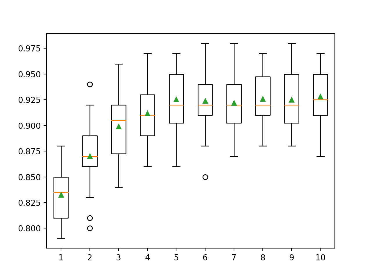
There are two main ways to control the complexity of a tree: through the maximum tree depth and the maximum number of terminal nodes (leaves) of the tree. We are examining the number of leaves here, so we need to increase the number to support deeper trees by specifying the num_leaves argument . Below we examine tree depths from 1 to 10 and their impact on model performance.
# explore lightgbm tree depth effect on performance
from numpy import mean
from numpy import std
from sklearn.datasets import make_classification
from sklearn.model_selection import cross_val_score
from sklearn.model_selection import RepeatedStratifiedKFold
from lightgbm import LGBMClassifier
from matplotlib import pyplot

# get the dataset
def get_dataset():
X, y = make_classification(n_samples=1000, n_features=20, n_informative=15, n_redundant=5, random_state=7)
return X, y

# get a list of models to evaluate
def get_models():
models = dict()
for i in range(1,11):
models[str(i)] = LGBMClassifier(max_depth=i, num_leaves=2**i)
return models

# evaluate a give model using cross-validation
def evaluate_model(model):
cv = RepeatedStratifiedKFold(n_splits=10, n_repeats=3, random_state=1)
scores = cross_val_score(model, X, y, scoring='accuracy', cv=cv, n_jobs=-1)
return scores

# define dataset
X, y = get_dataset()
# get the models to evaluate
models = get_models()
# evaluate the models and store results
results, names = list(), list()
for name, model in models.items():
scores = evaluate_model(model)
results.append(scores)
names.append(name)
print('>%s %.3f (%.3f)' % (name, mean(scores), std(scores)))
# plot model performance for comparison
pyplot.boxplot(results, labels=names, showmeans=True)
pyplot.show()
Running the example first displays the average precision for each adjusted tree depth.
Note : Your results may differ due to the stochastic nature of the algorithm or estimation procedure, or differences in numerical precision. Consider running the example several times and comparing the average result.
Here we can see that performance improves with increasing tree depth, possibly up to 10 levels. It would be interesting to explore even deeper trees.
>1 0.833 (0.028)
>2 0.870 (0.033)
>3 0.899 (0.032)
>4 0.912 (0.026)
>5 0.925 (0.031)
>6 0.924 (0.029)
>7 0.922 (0.027)
>8 0.926 (0.027)
>9 0.925 (0.028)
>10 0.928 (0.029)
A rectangle and whisker plot is generated to distribute the accuracy scores for each configured tree depth. There is a general tendency for the model performance to increase with a tree depth of up to five levels, after which the performance remains fairly flat.
Learning rate research
The learning rate controls the degree to which each model contributes to ensemble prediction. Lower speeds may require more decision trees in the ensemble. The learning rate can be controlled with the learning_rate argument, by default it is 0.1. The following examines the learning rate and compares the effect of values between 0.0001 and 1.0.
# explore lightgbm learning rate effect on performance
from numpy import mean
from numpy import std
from sklearn.datasets import make_classification
from sklearn.model_selection import cross_val_score
from sklearn.model_selection import RepeatedStratifiedKFold
from lightgbm import LGBMClassifier
from matplotlib import pyplot

# get the dataset
def get_dataset():
X, y = make_classification(n_samples=1000, n_features=20, n_informative=15, n_redundant=5, random_state=7)
return X, y

# get a list of models to evaluate
def get_models():
models = dict()
rates = [0.0001, 0.001, 0.01, 0.1, 1.0]
for r in rates:
key = '%.4f' % r
models[key] = LGBMClassifier(learning_rate=r)
return models

# evaluate a give model using cross-validation
def evaluate_model(model):
cv = RepeatedStratifiedKFold(n_splits=10, n_repeats=3, random_state=1)
scores = cross_val_score(model, X, y, scoring='accuracy', cv=cv, n_jobs=-1)
return scores

# define dataset
X, y = get_dataset()
# get the models to evaluate
models = get_models()
# evaluate the models and store results
results, names = list(), list()
for name, model in models.items():
scores = evaluate_model(model)
results.append(scores)
names.append(name)
print('>%s %.3f (%.3f)' % (name, mean(scores), std(scores)))
# plot model performance for comparison
pyplot.boxplot(results, labels=names, showmeans=True)
pyplot.show()
Running the example first displays the average accuracy for each configured learning rate.
Note : Your results may vary due to the stochastic nature of the algorithm or estimation procedure, or differences in numerical precision. Consider running the example multiple times and comparing the average result.
Here we see that a higher learning rate leads to better performance on this dataset. We expect that adding more trees to the ensemble for a lower learning rate will further improve performance.
>0.0001 0.800 (0.038)
>0.0010 0.811 (0.035)
>0.0100 0.859 (0.035)
>0.1000 0.925 (0.031)
>1.0000 0.928 (0.025)
A mustache box is created to distribute the accuracy scores for each configured learning rate. There is a general tendency for the model performance to increase with an increase in the learning rate up to 1.0.

Boosting type research
The peculiarity of LightGBM is that it supports a number of boosting algorithms called boost types. The boosting type is specified using the boosting_type argument and takes a string to determine the type. Possible values:
- 'gbdt' : Gradient Boosted Decision Tree (GDBT);
- 'dart' : the concept of dropout is entered into MART, we get DART;
- 'goss' : Gradient one-way fetch (GOSS).
The default is GDBT, the classic gradient boosting algorithm.
DART is described in a 2015 article titled " DART: Dropouts meet Multiple Additive Regression Trees " and, as the name suggests, adds the concept of deep learning dropout to the Multiple Additive Regression Trees (MART) algorithm, a precursor to gradient boosting decision trees.
This algorithm is known by many names, including Gradient TreeBoost, Boosted Trees, and Multiple Additive Regression Trees and Trees (MART). We use the latter name to refer to the algorithm.
GOSS is presented with work on LightGBM and the lightbgm library. This approach aims to use only those instances that result in a large error gradient to update the model and remove the remaining instances.
... We exclude a significant part of the data instances with small gradients and use only the rest to estimate the increase in information.
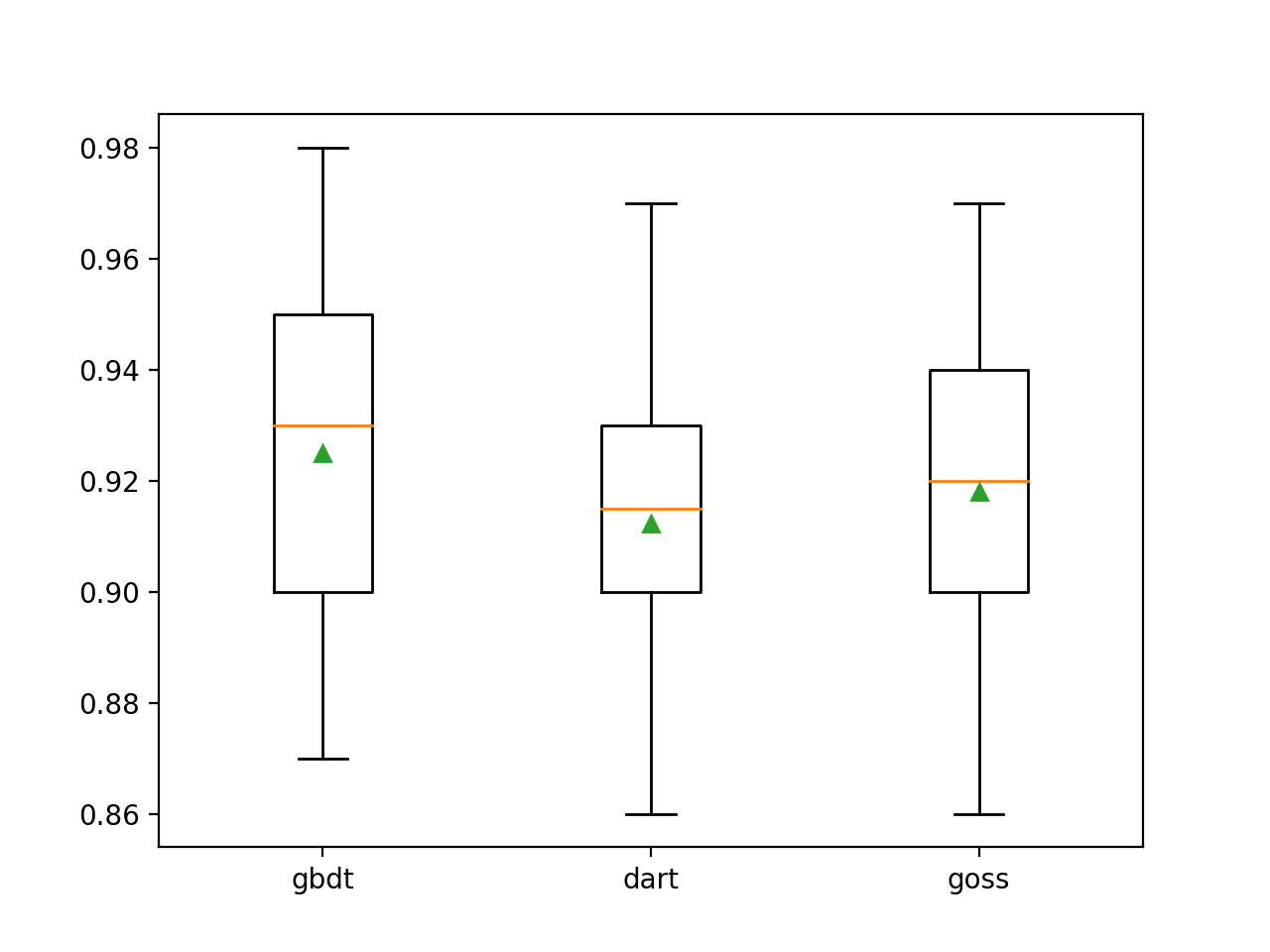
Below LightGBM is trained on a synthetic classification dataset with three key boosting methods.
# explore lightgbm boosting type effect on performance
from numpy import arange
from numpy import mean
from numpy import std
from sklearn.datasets import make_classification
from sklearn.model_selection import cross_val_score
from sklearn.model_selection import RepeatedStratifiedKFold
from lightgbm import LGBMClassifier
from matplotlib import pyplot

# get the dataset
def get_dataset():
X, y = make_classification(n_samples=1000, n_features=20, n_informative=15, n_redundant=5, random_state=7)
return X, y

# get a list of models to evaluate
def get_models():
models = dict()
types = ['gbdt', 'dart', 'goss']
for t in types:
models[t] = LGBMClassifier(boosting_type=t)
return models

# evaluate a give model using cross-validation
def evaluate_model(model):
cv = RepeatedStratifiedKFold(n_splits=10, n_repeats=3, random_state=1)
scores = cross_val_score(model, X, y, scoring='accuracy', cv=cv, n_jobs=-1)
return scores

# define dataset
X, y = get_dataset()
# get the models to evaluate
models = get_models()
# evaluate the models and store results
results, names = list(), list()
for name, model in models.items():
scores = evaluate_model(model)
results.append(scores)
names.append(name)
print('>%s %.3f (%.3f)' % (name, mean(scores), std(scores)))
# plot model performance for comparison

pyplot.boxplot(results, labels=names, showmeans=True)
pyplot.show()
Running the example first displays the average accuracy for each configured boost type.
Note : Your results may differ due to the stochastic nature of the algorithm or estimation procedure, or differences in numerical precision. Consider running the example several times and comparing the average result.
We can see that the default boost method performs better than the other two evaluated methods.
>gbdt 0.925 (0.031)
>dart 0.912 (0.028)
>goss 0.918 (0.027)
A box-and-whisker diagram is created to distribute the accuracy scores for each configured amplification method, allowing direct comparison of the methods.

- Machine Learning Course
- Data Science profession training
- Data Analyst training
- Python for Web Development Course
More courses
- Advanced Course "Machine Learning Pro + Deep Learning"
- Course "Mathematics and Machine Learning for Data Science"
- Profession Ethical hacker
- Unity Game Developer
- JavaScript course
- Profession Web developer
- Java-
- C++
- DevOps
- iOS-
- Android-
Recommended articles
- How Much Data Scientist Earns: An Overview of Salaries and Jobs in 2020
- : 2020
- Data Scientist -
- 450
- Machine Learning 5 9
- Machine Learning Computer Vision
- Machine Learning Computer Vision