Introduction
This article is about how we, together with the Rosneft subsidiary Samaraneftekhimproekt and the Kazan Federal University, held the Hackathon of Three Cities in September 2020, where we invited students to solve the classic problem of seismic correlation of reflecting horizons. These are the challenges that seismic professionals around the world face on a daily basis. For the participants, the task was decided to be presented as “the task of finding the optimal path” so as not to scare away the students with terrible words. In the article, we will tell you more about the problem and analyze interesting solutions of the participants. It will be exciting for both applied mathematical modeling and machine learning and data analysts.
Organizational part
We told interesting details of organizing an online hackathon in three cities in an article on vc.ru - Oil and Hackathon. A marathon isn't just about running .
We will only mention that for the online format we have chosen the Discord service and will leave a link to the hackathon rules (link on the Boosters site ).
Formulation of the problem
In seismic exploration, there is the concept of "seismic reflecting horizon" - this is a stable reflected wave in terms of dynamics and propagation area, which corresponds to a certain geological boundary. Correctly processing the field seismic data and recognizing (seismic prospecting experts say - "interpreting") seismic horizons, it is possible to determine the depth of their occurrence with an accuracy of 5-10 meters. Having determined the depths, then it is possible, together with geologists, to tie these horizons to the geochronological scale ( Geochronological scale - Wikipedia ) and recognize their smaller counterparts. And then decide - between which horizons the oil traps can lie, what the relief of the structural model of the field looks like, etc.
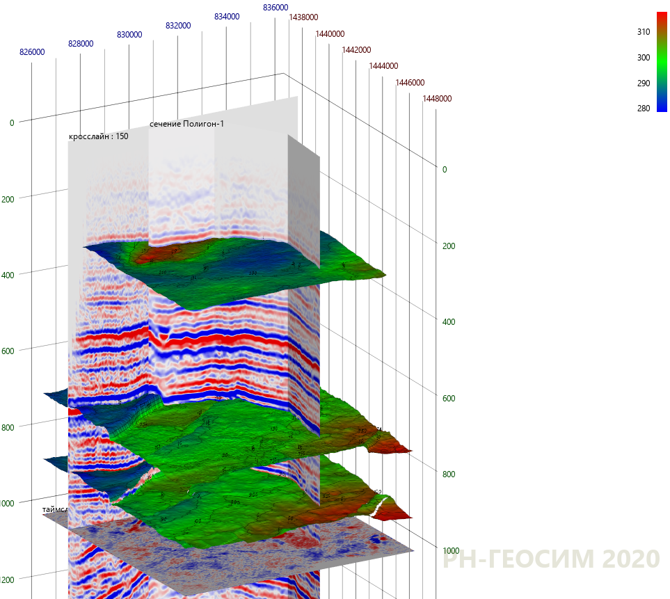
Vertical sections of the seismic cube and recognized seismic reflecting horizons
In practice, horizons are identified layer by layer on the seismic sections of the seismic cube - both manually, using an array (seismic experts say - "diving") a large number of reference points, and using automated and semi-automated search procedures ... Of course, a high-quality solution to the problem of interpreting seismic horizons using software is in great demand and can significantly reduce the time spent by seismic prospecting specialists.
At the same time, the study of sources ( Least-squares horizons with local slopes and multi-grid correlations, Waveform Embedding: automatic horizon picking with unsupervised deep learning) shows that the developed algorithms and solutions are based on a small number of mathematical approaches, so we decided to try to attract students with their consciousness not yet clouded by scientific research and offer them this problem in the form of a problem of finding the optimal path on a complex surface.
As a result, the problem was formulated as follows: construction of a path of motion on a complex surface passing through given points and satisfying the conditions of a minimum of a certain functional depending on the length of the path and its angles (gradients).
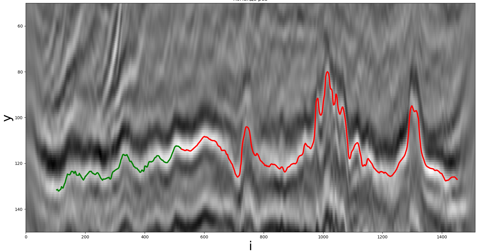
An example of a portion of the original seismic section for building a horizon. The green line is the previously known part, the red line is the required part.
The participants of the competition had to find a solution in 12 hours that would allow them to continue their path along the optimal trajectory on the hidden part of the dataset. There were 20 attempts to validate the solution; the participant with the minimum metric value won.
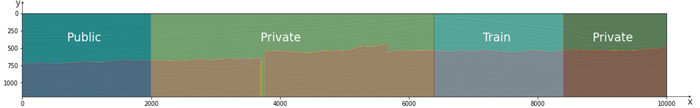
Detailed data description
, :
, – 2 .
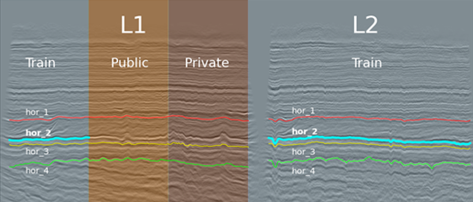
-, hor_2 L1. L2 L1. . , , .
- . , [x,y] z(x,y) .
- (x,y) L1 L2. x, hor_1, …, hor_4.
- L2 4 (1, 2, 3, 4), L1 – 3 (1, 3, 4). 2- L1 (40%). 60% .
, – 2 .
-, hor_2 L1. L2 L1. . , , .
Throughout the competition, the standings were built based on the metric values on the public part of the test data. After the end of the competition, the metric value was recalculated in the private part, and the standings were updated. This is important in order to obtain sustainable solutions, that is, not only tailored to public data, but also capable of showing a comparable result on private data. It turned out that this was not done in vain, and after the final quality assessment, the standings changed.
The following metric was used to quantify the results obtained:
where:
N is the dimension of the required horizon;
- the coordinates of the horizon, obtained using the algorithm, ;
- coordinates of the reference horizon;
- values of the surface map at the point with coordinates i, yi;
, where height is the maximum possible value of the y coordinate of the surface map;
where max (z) is the largest value of the surface map.
Metric implementation in Python
def score(true, submission, all_data):
   #true – pandas.Dataframe    ;
   #submission - pandas.Dataframe   ,
   #;
   #all_data - numpy.ndarray
   all_data = all_data.astype('float64')
   #
   max_z = abs(all_data).max()
   #
   y_pred = submission.loc[idx.index.values].y.values.astype('int')
   #
   y_true = true.y.astype(int)
   #
   z_pred = all_data[true.index.values.astype(int), y_pred.astype(int)]
   #
   z_true = all_data[true.index.values, y_true]
   #
   y_err = ((y_pred - y_true)/3000)** 2
   z_err = ((z_pred - z_true)/max_z) ** 2
   #
   total_err = np.sqrt(np.sum(y_err + z_err))
   return total_err
What methods were used by the teams
The problem was initially selected such that it could be solved in several ways: direct and inverse (using classical mathematical methods and machine learning methods, respectively).
From the point of view of machine learning, the problem can be solved by two methods:
1) Construction of regression
Using known pairs of points (), you can construct a mapping by minimizing the loss function L. - indicative description of the i-th point.
For instance, or
The loss function can be either the initial error function from the problem statement, or a simpler function, for example, the standard deviation of the constructed and original paths:
Many popular machine learning methods can be used to construct the mapping f : starting with polynomial regression, traversing a random forest, and deep neural networks.
Several teams have taken this approach using asconvolutional or fully connected neural network, and as f - neural network or Gaussian processes.
2) Semantic segmentation
An example of semantic segmentation
The original problem can be solved as a computer vision problem. Points (x, y) are considered as image pixels, where the entire image is the entire dataset, and the "brightness" of the pixel (x, y) is the z (x, y) value. To build a path, you need to assign one of the classes to each pixel - 0 or 1. The part of the image that is below the path or includes it belongs to class 0, and the rest - to class 1. A household solution for such a problem is a fully convolutional neural network U-Net, on an input that receives a piece (patch) of the original image and outputs an array of the same size, consisting of zeros and ones, denoting the classes of the corresponding pixels.
In addition to deep learning techniques, you can also use classical computer vision and image processing techniques such as Flood fill for image segmentation. This was done by one of the participants, thereby pre-processing the image for further application of algorithms for finding the shortest path.
From the point of view of classical mathematical methods, the proposed problem is a classical optimization problem, and we observed attempts to solve it by the following groups of methods:
- , ;
. y , y, . - , ;
. - , .
, .
First, let's analyze the decisions of the participants.
Machine learning methods:
One of the solutions was an autoregressive convolutional neural network that produces a real number - the value of the pathfor the i-th step. The 32x32 pixel patches of the original image were fed to the input of the neural network. As a functionFor feature extraction, the pretrained convolutional neural network ResNet34 was used. The feature representation obtained by this neural network was combined with the values of this path from the previous 32 steps. To predict further 32 steps, previous neural network predictions were used as the previous horizon values. The neural network was trained by a modification of Adam stochastic gradient descent with an exponential decrease in the optimizer step as it is trained. For training, the mean absolute deviation was minimized (experiments with the standard deviation gave worse results). To avoid overfitting, a Dropout was used, that is, random zeroing of a part of neurons. It took about 10 minutes to train the neural network, 20 full passes over the entire dataset and 720 optimizer steps.
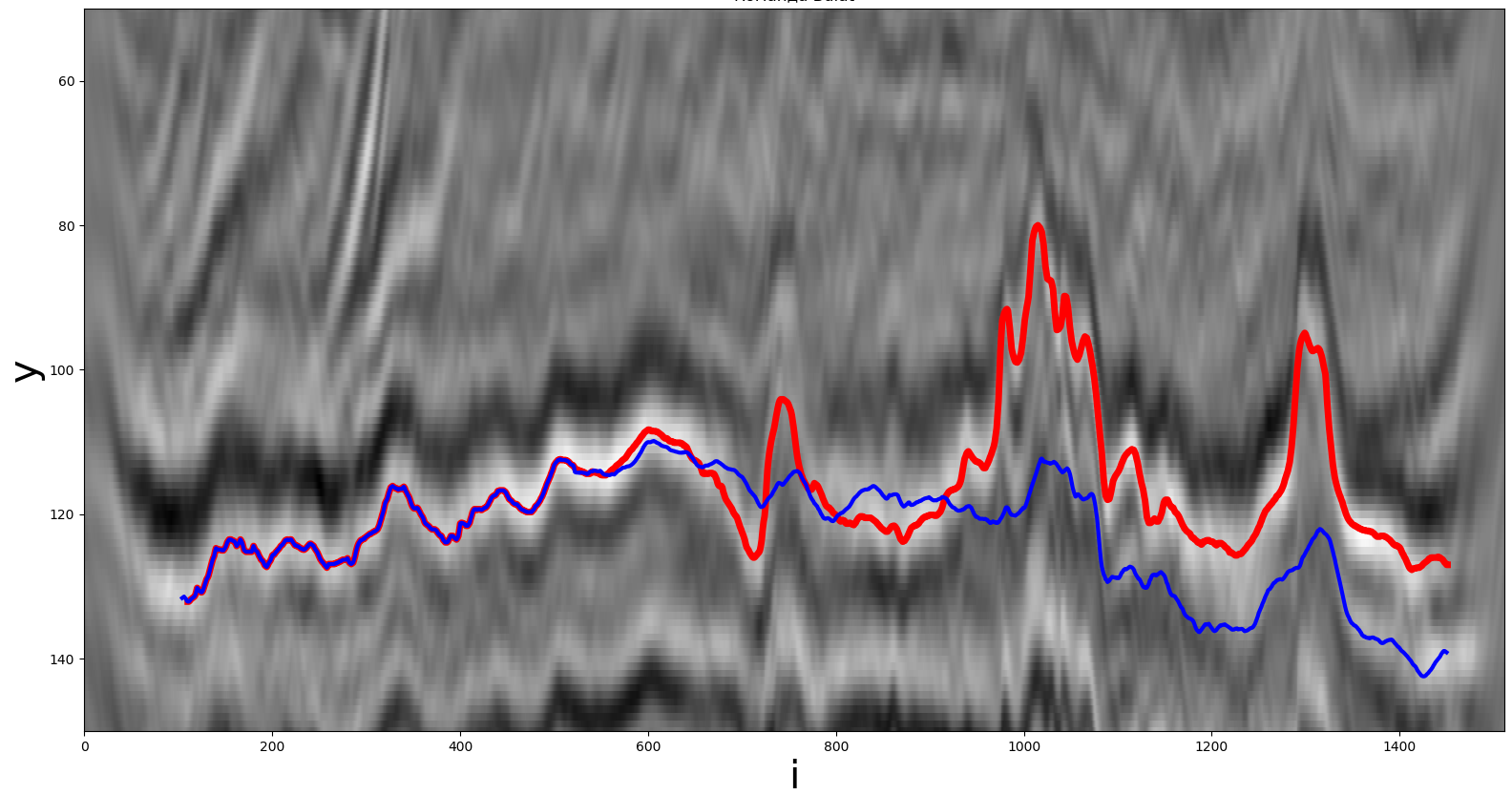
A solution obtained using a convolutional neural network. The red line is the real path, the blue line is the one received by the participant.
Neural network prediction takes about 1 minute on an AMD Threadripper 2950x CPU and an Nvidia GTX 1080 Ti GPU.
The result of the neural network (metric) is 5.71 on the public standings. Experiments were also done with replacing the convolutional neural network with a recurrent one, but its result was worse. As a result, classical methods of computational mathematics were used as the final solution.
In addition to finished solutions, the participants also shared their ideas, which they did not manage to implement due to the tight time frame of the competition and the computational complexity of their ideas. Some of them tried to apply neural networks, but after spending most of their time, they moved on to simpler and more efficient algorithms or even to brute force and rules, which ultimately gave the best result and led to prizes.
Also, a number of interesting solutions are based on knowledge from other disciplines: for example, classical computer vision and image processing, graph theory, time series analysis. One of the teams even posed a challenge in terms of reinforcement learning that you might have heard of, and came up with a solution, but unfortunately didn't have time to implement it.
Classical mathematical methods:
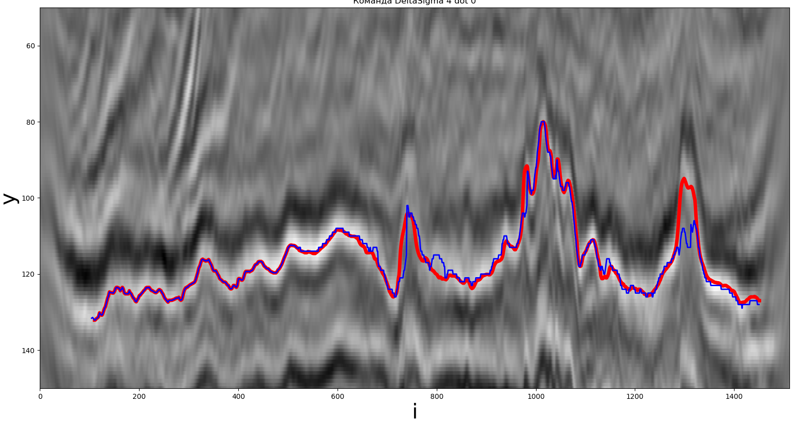
One of the solutions obtained by the local extremum method. The red line is the real path, the blue line is the one received by the participant.
For this method, a local maximum was used as an extremum. The path built by the participants is marked in blue, the desired horizon is in red. A detailed description is provided below.
,
,
,
Where:
- the maximum possible value of the y coordinate of the surface map;
- the size of the search window.
The method is implemented in Python. The operating time was about 0.103 seconds, F (y, z) = 1.57,= 100.
Conclusion: the method is simple enough to implement, the running time does not exceed 0.1 seconds.
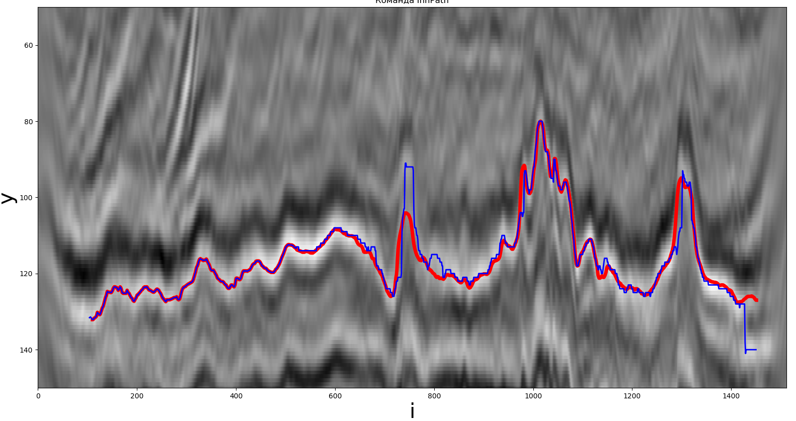
One of the solutions obtained by the global extremum. The red line is the real path, the blue line is the one received by the participant.
Let's move on to the next group. As before, in this method, the maximum was used as the extreme.
,
,
,
where:
height is the maximum possible value of the y coordinate of the surface map;
- the size of the search window.
The method is implemented in Python. The operating time was about 0.19 seconds, F (y, z) = 1.97,= 9, = 21.
Conclusion: the method is simple enough to implement, the running time does not exceed 0.2 seconds.
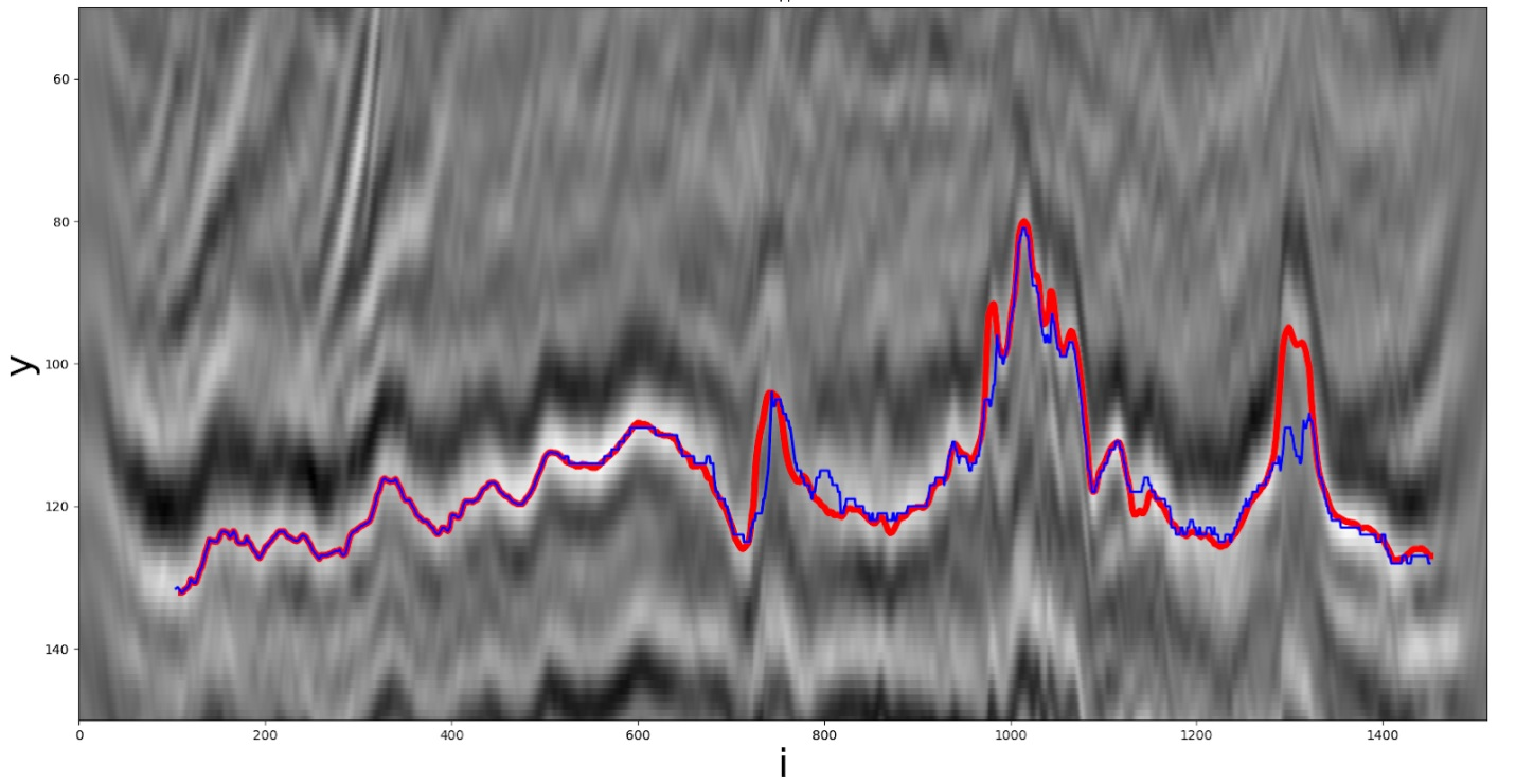
One of the heuristic solutions. The red line is the real path, the blue line is the one received by the participant.
Let's consider the last group of methods. As mentioned earlier, the next coordinateis searched for by the minimum of functionality within the specified search window.
Below is one of the functionalities proposed by the teams. From a mathematical point, it looks like this:
,
,
Where:
- the maximum possible value of the y coordinate of the surface map;
- coefficient responsible for the influence of the error in y on the value of the functional;
- the size of the search window;
Is the highest value of the surface map.
The method was implemented in Python. The operating time was about 0.12 seconds, F (y, z) = 1.58,= 50, = 15000.7.
Conclusion: the running time of the method does not exceed 0.15 seconds.
The methods of all three groups showed fairly similar results on a given dataset. The smallest metric value (1.57) was achieved by a method based on the search for local extrema of surface values within a given search window.
Final part
Unfortunately, by the end of the hackathon, almost all innovators had
We wanted to bring together contributors from two areas: computational mathematics and machine learning. Some are accustomed to working with unstructured data of unknown nature, others - to study physical processes and build mathematical models on their basis. To increase the variety of ideas and solutions, we briefly described how the data was obtained. This is one of the reasons why the solution based on simple numerical methods gave the best results. The second reason was that for the student hackathon, we prepared not very "complex" data of a small volume, so modern time-consuming machine learning methods lose out to simpler alternatives.
We believe that this is a great lesson that will help participants to correctly set problems and choose the best methods for solving them. It is important to remember that first you should try a simple solution, the so-called baseline, perhaps it will allow you to achieve your goal in a short time.
The Hackathon participants proposed their own algorithms for finding the optimal path in a big data set in relation to the problem of automatic seismic kinematic interpretation, which is currently being solved as part of the development of corporate software in the field of geology and seismics. The most competitive implementations of algorithms will find their application in the development and implementation of software modules for these software systems.
We will be glad to see you at the final of the IT competition marathon, which will be held on November 28 online. The program includes: rewarding the winners of the competition, presentation of the first version of the mobile application for express assessment of the proppant quality. Also within the framework of the event, panel discussions will be organized on topical topics "Data and DS Projects Management" and "Computer Vision". Representatives of Head of Data Science Alfa, CDO Megafon, Huawei, Head of CV X5 and others will share interesting cases. Do not miss all the fun ( IT Competition Marathon 2020 - Rosneft ).