Control of multi-link manipulators of a robotic complex using a neural network

Introduction

When simulating motion control systems for robots, it is required to solve the problems of kinematics and dynamics for their actuators. There is an inverse and a direct problem of kinematics. The direct problem of kinematics is to determine the spatial position and orientation of the characteristic point, as a rule, of the working tool of the robot manipulator by the known values ​​of the generalized coordinates. The inverse problem of kinematics, like the direct problem, is one of the main problems of kinematic analysis and synthesis. To control the position of the links and the orientation of the working tool of the manipulator, it becomes necessary to solve the inverse problem of kinematics.

Most of the analytical approaches for solving the inverse kinematics problem are quite expensive in terms of computational procedures. One of the alternative approaches is the use of neural networks. Input data. Consider a three-link manipulator with the parameters shown in Table 1.

Table 1 - DH parameters for a three-link manipulator

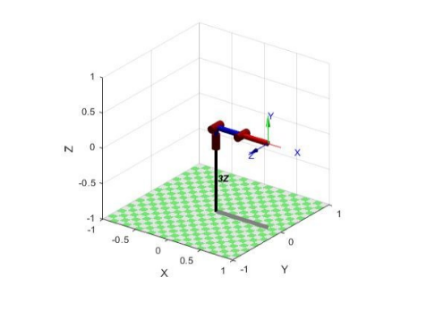
In the MatLab environment, using the free Robotics Toolbox, a computer model of a three-link manipulator is built. Below is a fragment of the MatLab script in which we assign to the 'L' array the values ​​of the parameters, A, Alfa, and D from Table 1. For our model, these are constant values ​​and they do not change in the process of working with the manipulator. We assign the Tetta parameter to the variable 'initialPose_left' - the initial position of our manipulator. 

function [L,initialPose_left,baseL] =model3z 
%   
initialPose_left = deg2rad([0 0 0]); 
L(1) = Revolute('d', 0.2, 'alpha', pi/2, 'qlim', initialPose_left(1)+deg2rad([-90 +90]) ); 
L(2) = Revolute('d', 0, 'alpha', 0, 'a', 0.4, 'qlim', initialPose_left(2)+deg2rad([-20 +90]));   
L(3) = Revolute('d', 0, 'alpha', 0, 'a', 0.4, 'qlim', initialPose_left(2)+deg2rad([-90 +90])); 
% -178 +178 
baseL = [1 0 0 0;  
        0 1 0 0;  
        0 0 1 0;  
        0 0 0 1]; 

1 (. 1) . 

 Tetta, .  initialPose_left. 

. , . 

, .  

  . :

q – . 

%       
t1_min = L(1).qlim(1); t1_max = L(1).qlim(2);  
t2_min = L(2).qlim(1); t2_max = L(2).qlim(2); 
t3_min = L(3).qlim(1); t3_max = L(3).qlim(2); 
%     
t1 = t1_min + (t1_max-t1_min)*rand(N,1); 
t2 = t2_min + (t2_max-t2_min)*rand(N,1); 
t3 = t3_min + (t3_max-t3_min)*rand(N,1); 
Y = horzcat(t1, t2, t3);

, .  : 

:  x,y,z – . R – , . 

%    4x4 
T = zeros(4, 4, N); 
T(:, :, :) = leftArm.fkine(Y); %  ,       
%R = tr2rpy(T(1:3, 1:3, :), 'arm'); %      
R = tr2eul(T(1:3, 1:3, :)); %      
Tx = reshape(T(1, 4, :), [N 1]); %  - 
Ty = reshape(T(2, 4, :), [N 1]); 
Tz = reshape(T(3, 4, :), [N 1]); 
% scatter3(Tx,Ty,Tz,'.','r'); 
X = horzcat(Tx, Ty, Tz, R); %   

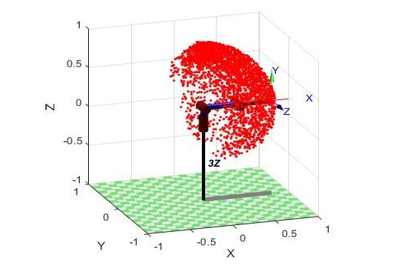
. 3.2.1  , 3000 . 

, 3000 . , X Y. 

, .

Keras Python. .

X_train, X_test, y_train, y_test = train_test_split(data_x, data_y, test_size=0.2,
random_state=42) 

« » . .

def base_model():
 model = Sequential()
 model.add(Dense(32,input_dim=6,activation='relu'))
 model.add(Dense(64,activation='relu'))
 model.add(Dense(128,activation='relu'))
 model.add(Dense(32,activation='relu'))
 model.add(Dense(3, init='normal'))
 model.compile(loss='mean_absolute_error', optimizer = 'adam', metrics=['accuracy'])
 model.summary()
 return model

, . . , , . , , .       KerasRegressor,  Keras.

clf = KerasRegressor(build_fn=base_model, epochs=500, batch_size=20,verbose=2)
clf.fit(X_train,y_train) 

.

res = clf.predict(X_test) 

99% , . 

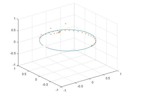
3 , , , . . , . . - . , , , , .

%%    ,    
M=[-178:10:178]; %      -178   +178    10 
M_size=length(M); 
first_q=zeros(M_size, 3); 
T33 = zeros(4, 4, M_size); 
T34 = zeros(4, 4, M_size); 
first_q(:,1)=[deg2rad(M)]; %  q 
T33(:, :, :) = leftArm.fkine(first_q);%      ,   
R = tr2rpy(T33(1:3, 1:3, :), 'arm'); %      
Tx = reshape(T33(1, 4, :), [M_size 1]); %  - 
Ty = reshape(T33(2, 4, :), [M_size 1]); 
Tz = reshape(T33(3, 4, :), [M_size 1]); 
plot3(Tx,Ty,Tz) 
axis([-1 1 -1 1 -1 1]);hold on;grid on; 

XX = horzcat(Tx, Ty, Tz, R); %        
T34(:, :, :) = leftArm.fkine(q_new); %     ,   
Tx2 = reshape(T34(1, 4, :), [M_size 1]); %  - 
Ty2 = reshape(T34(2, 4, :), [M_size 1]); 
Tz2 = reshape(T34(3, 4, :), [M_size 1]); 
plot3(Tx2,Ty2,Tz2,'.') 
axis([-1 1 -1 1 -1 1]) 

. . , - . , . . «Programming by demonstration», . Matlab , – .