What was the purpose of this study? I wanted to know:
- In what applications is Python used
- What knowledge is required: databases, libraries, frameworks
- How much specialists in each area are in demand
- What salaries are offered

Loading data
Jobs downloaded from the site hh.ru , using the API: dev.hh.ru . At the request of "Python", 1994 vacancies were uploaded (Moscow region), which were divided into training and test suites, in the proportion of 80% and 20% . The size of the training set is 1595 , the size of the test set is 399 . The test set will only be used in the Top / Antitop skills and Job Classification sections.
Signs
Based on the text of uploaded vacancies, two groups of the most common n-grams of words were formed :
- 2-grams in Cyrillic and Latin
- 1-grams in Latin
In IT vacancies, key skills and technologies are usually written in English, so the second group included words only in Latin.
After selection of the first n-gram group contained 81 grams of 2, 1 and the second 98-gram:
| No. | n | n-gram | Weight | Vacancies |
| 1 | 2 | in python | eight | 258 |
| 2 | 2 | ci cd | eight | 230 |
| 3 | 2 | understanding of principles | eight | 221 |
| 4 | 2 | knowledge of sql | eight | 178 |
| five | 2 | development and | nine | 174 |
| ... | ... | ... | ... | ... |
| 82 | 1 | sql | five | 490 |
| 83 | 1 | linux | 6 | 462 |
| 84 | 1 | postgresql | five | 362 |
| 85 | 1 | docker | 7 | 358 |
| 86 | 1 | java | nine | 297 |
| ... | ... | ... | ... | ... |
It was decided to divide vacancies into clusters according to the following criteria, in order of priority:
| A priority | Criterion | Weight |
| 1 | Field (applied direction), position,
n-gram experience : "machine learning", "linux administration", "excellent knowledge" |
7-9 |
| 2 | Tools, technologies, software.
n-grams: "sql", "linux os", "pytest" |
4-6 |
| 3 | Other
n-gram skills : "technical education", "English", "interesting tasks" |
1-3 |
Determination of which group of criteria the n-gram belongs to, and what weight to assign to it, occurred on an intuitive level. Here are a couple of examples:
- At first glance, "Docker" can be attributed to the second group of criteria with a weight of 4 to 6. But the mention of "Docker" in the vacancy most likely means that the vacancy will be for the position of "DevOps engineer". Therefore, "Docker" fell into the first group and received a weight of 7.
- «Java» , .. «Java» Java- « Python». «-». , , , «Java» 9.
n- — .
For calculations, each vacancy was transformed into a vector with a dimension of 179 (the number of selected features) of integers from 0 to 9, where 0 means that the i-th n-gram is absent in the vacancy, and the numbers from 1 to 9 mean the presence of the i-th n - grams and its weight. Further in the text, a dot means a vacancy represented by such a vector.
Example:
Let's say the list of n-grams contains only three values:
No. n n-gram Weight Vacancies 1 2 in python eight 258 2 2 understanding of principles eight 221 3 1 sql five 490
Then for a vacancy with text.
Requirements:
- 3+ years of experience in python development .
- Good knowledge of sql
the vector is equal to [8, 0, 5].
Metrics
To work with data, you need to have an understanding of it. In our case, I would like to see if there are any clusters of points, which we will consider as clusters. To do this, I used the t-SNE algorithm to translate all vectors into 2D space.
The essence of the method is to reduce the dimension of the data, while keeping the proportions of the distances between the points of the set as much as possible. It is quite difficult to understand how t-SNE works from the formulas. But I liked one example found somewhere on the Internet: let's say we have balls in three-dimensional space. We connect each ball with all other balls by invisible springs, which do not intersect in any way and do not interfere with each other when crossing. The springs act in two directions, i.e. they resist both the distance and the approach of the balls to each other. The system is in a stable state, the balls are stationary. If we take one of the balls and pull it back, and then release it, it will return to its original state due to the force of the springs. Next, we take two large plates, and squeeze the balls into a thin layer,while not interfering with the balls to move in the plane between the two plates. The forces of the springs begin to act, the balls move and eventually stop when the forces of all the springs become balanced. The springs will act so that the balls that were close to each other remain relatively close and flat. Also with removed balls - they will be removed from each other. With the help of springs and plates, we converted the three-dimensional space into two-dimensional, preserving the distance between the points in some form!Also with removed balls - they will be removed from each other. With the help of springs and plates, we converted the three-dimensional space into two-dimensional, preserving the distance between the points in some form!Also with removed balls - they will be removed from each other. With the help of springs and plates, we converted the three-dimensional space into two-dimensional, preserving the distance between the points in some form!
T-SNE algorithm used by me only for visualization of the set points. He helped choose the metric, as well as select the weights for the features.
If we use the Euclidean metric that we use in our daily life, then the location of vacancies will look like this:

The figure shows that most of the points are concentrated in the center, and there are small branches to the sides. With this approach, clustering algorithms that use the distances between points will not produce anything good.
There are many metrics (ways to determine the distance between two points) that will work well on the data you are exploring. I have chosen as a measure of the distance Jaccard , taking into account the weights of n-grams. Jaccard's measure is easy to understand, but it works well for solving the problem under consideration.
:
1 n-: « python», «sql», «docker»
2 n-: « python», «sql», «php»
:
« python» — 8
«sql» — 5
«docker» — 7
«php» — 9
(n- 1- 2- ): « python», «sql» = 8 + 5 = 13
( n- 1- 2- ): « python», «sql», «docker», «php» = 8 + 5 + 7 + 9 = 29
=1 — ( / ) = 1 — (13 / 29) = 0.55
The matrix of distances between all pairs of points was calculated, the size of the matrix is 1595 x 1595. In total, 1,271,215 distances between unique pairs. The average distance turned out to be 0.96, between 619 659 the distance is 1 (i.e. there is no similarity at all). The following chart shows that overall vacancies are few similarities:
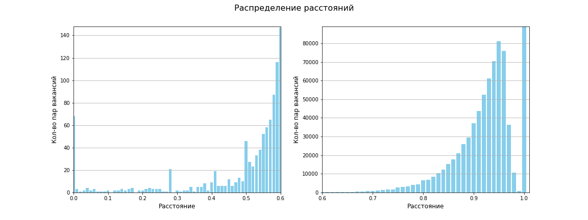
When using the metric Jaccard our space now looks like this:

Four distinct areas of density appeared, and two small clusters of low density. At least that's how my eyes see!
Clustering
The model was chosen as a clustering algorithm Gaussian Mixture Model (GMM) . The algorithm receives data in the form of vectors as input, and the n_components parameter is the number of clusters into which the set must be split. About how the algorithm works, you can see here (in English). I used a ready-made GMM implementation from the scikit-learn library: sklearn.mixture.GaussianMixture .
Note that GMM does not use a metric, but separates data only by a set of features and their weights. In the article, Jaccard distance is used to visualize data, calculate the compactness of clusters (I took the average distance between cluster points for compactness), and determinethe central point of the cluster (typical vacancy) - the point with the smallest average distance to other points of the cluster. Many clustering algorithms use exactly the distance between points. The Other Methods section will talk about other types of clustering that are metric-based and also give good results.
In the previous section, it was determined by eye that there will most likely be six clusters. This is how the clustering results look with n_components = 6:

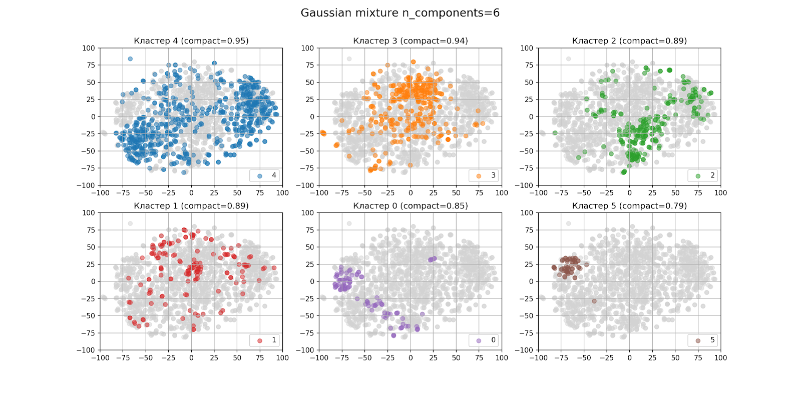
In the figure with the output of clusters separately, the clusters are arranged in descending order of the number of points from left to right, from top to bottom: cluster 4 is the largest, cluster 5 is the smallest. The compactness of each cluster is indicated in brackets.
In appearance, the clustering turned out to be not very good, even considering that the t-SNE algorithm is not perfect. When analyzing clusters, the result was also not encouraging.
To find the optimal number of clusters n_components, we will use the AIC and BIC criteria , which you can read about here . The calculation of these criteria is built into the sklearn.mixture.GaussianMixture method . This is how the criteria graph looks like:

When n_components = 12, the BIC criterion has the lowest (best) value, the AIC criterion also has a value close to the minimum (minimum when n_components = 23). Let's divide vacancies into 12 clusters:


Clusters are now more compact, both in appearance and in numerical terms. During manual analysis, vacancies were divided into characteristic groups for understanding a person. The figure shows the names of the clusters. Clusters numbered 11 and 4 are marked as <Trash 2>:
- In cluster 11, all features have approximately the same total weights.
- Cluster 4 is dedicated to Java. Nevertheless, there are few vacancies for the position of Java Developer in the cluster, knowledge of Java is often required as "will be an additional plus."
Clusters
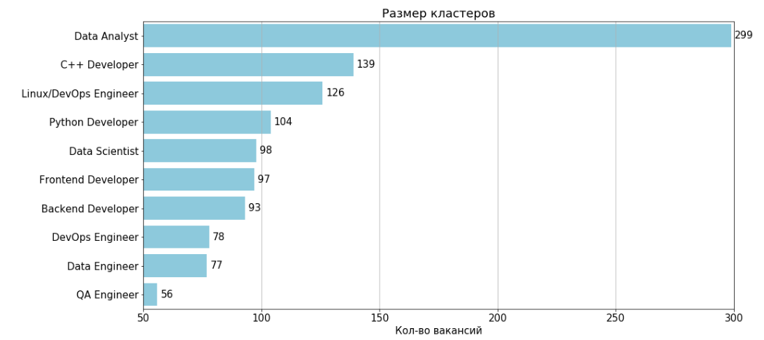
After deleting two uninformative clusters numbered 11 and 4, the result is 10 clusters:
For each cluster, there is a table of features and 2-grams that are most often found in the vacancies of the cluster.
Legend:
S - the proportion of vacancies in which the trait is found, multiplied by the weight of the trait
% - the percentage of vacancies in which the trait / 2-gram is found
Typical cluster vacancy - vacancy, with the smallest average distance to other points of the cluster
Data Analyst
Number of Jobs: 299
Typical Job : 35,805,914
| No. | Sign with weight | S | Sign | % | 2-grams | % |
| 1 | excel | 3.13 | sql | 64.55 | knowledge of sql | 18.39 |
| 2 | r | 2.59 | excel | 34.78 | in developing | 14.05 |
| 3 | sql | 2.44 | r | 28.76 | python r | 14.05 |
| 4 | knowledge of sql | 1.47 | bi | 19.40 | with big | 13.38 |
| five | data analysis | 1.17 | tableau | 15.38 | development and | 13.38 |
| 6 | tableau | 1.08 | 14.38 | data analysis | 13.04 | |
| 7 | with big | 1.07 | vba | 13.04 | knowledge of python | 12.71 |
| eight | development and | 1.07 | science | 9.70 | analytical warehouse | 11.71 |
| nine | vba | 1.04 | dwh | 6.35 | development experience | 11.71 |
| ten | knowledge of python | 1.02 | oracle | 6.35 | databases | 11.37 |
C ++ Developer
Number of Jobs: 139
Typical Job : 39,955,360
| No. | Sign with weight | S | Sign | % | 2-grams | % |
| 1 | c ++ | 9.00 | c ++ | 100.00 | development experience | 44.60 |
| 2 | java | 3.30 | linux | 44.60 | c c ++ | 27.34 |
| 3 | linux | 2.55 | java | 36.69 | c ++ python | 17.99 |
| 4 | c # | 1.88 | sql | 23.02 | in c ++ | 16.55 |
| five | go | 1.75 | c # | 20.86 | development on | 15.83 |
| 6 | development on | 1.27 | go | 19.42 | data structures | 15.11 |
| 7 | good knowledge | 1.15 | unix | 12.23 | writing experience | 14.39 |
| eight | data structures | 1.06 | tensorflow | 11.51 | programming on | 13.67 |
| nine | tensorflow | 1.04 | bash | 10.07 | in developing | 13.67 |
| ten | programming experience | 0.98 | postgresql | 9.35 | programming languages | 12.95 |
Linux / DevOps Engineer
Number of Job Openings: 126
Typical Job : 39,533,926
| No. | Sign with weight | S | Sign | % | 2-grams | % |
| 1 | ansible | 5.33 | linux | 84.92 | ci cd | 58.73 |
| 2 | docker | 4.78 | ansible | 76.19 | administration experience | 42.06 |
| 3 | bash | 4.78 | docker | 74.60 | bash python | 33.33 |
| 4 | ci cd | 4.70 | bash | 68.25 | tcp ip | 39.37 |
| five | linux | 4.43 | prometheus | 58.73 | customization experience | 28.57 |
| 6 | prometheus | 4.11 | zabbix | 54.76 | monitoring and | 26.98 |
| 7 | nginx | 3.67 | nginx | 52.38 | prometheus grafana | 23.81 |
| eight | administration experience | 3.37 | grafana | 52.38 | monitoring systems | 22.22 |
| nine | zabbix | 3.29 | postgresql | 51.59 | with docker | 16.67 |
| ten | elk | 3.22 | kubernetes | 51.59 | configuration management | 16.67 |
Python Developer
Number of Job Openings: 104
Typical Job : 39,705,484
| No. | Sign with weight | S | Sign | % | 2-grams | % |
| 1 | in python | 6.00 | docker | 65.38 | in python | 75.00 |
| 2 | django | 5.62 | django | 62.50 | development on | 51.92 |
| 3 | flask | 4.59 | postgresql | 58.65 | development experience | 43.27 |
| 4 | docker | 4.24 | flask | 50.96 | django flask | 04.24 |
| five | development on | 4.15 | redis | 38.46 | rest api | 23.08 |
| 6 | postgresql | 2.93 | linux | 35.58 | python from | 21.15 |
| 7 | aiohttp | 1.99 | rabbitmq | 33.65 | databases | 18.27 |
| eight | redis | 1.92 | sql | 30.77 | writing experience | 18.27 |
| nine | linux | 1.73 | mongodb | 25.00 | with docker | 17.31 |
| ten | rabbitmq | 1.68 | aiohttp | 22.12 | with postgresql | 16.35 |
Data scientist
Number of vacancies: 98
Typical vacancy: 38071218
| No. | Sign with weight | S | Sign | % | 2-grams | % |
| 1 | pandas | 7.35 | pandas | 81.63 | machine learning | 63.27 |
| 2 | numpy | 6.04 | numpy | 75.51 | pandas numpy | 43.88 |
| 3 | machine learning | 5.69 | sql | 62.24 | data analysis | 29.59 |
| 4 | pytorch | 3.77 | pytorch | 41.84 | data science | 26.53 |
| five | ml | 3.49 | ml | 38.78 | knowledge of python | 25.51 |
| 6 | tensorflow | 3.31 | tensorflow | 36.73 | numpy scipy | 24.49 |
| 7 | data analysis | 2.66 | spark | 32.65 | python pandas | 23.47 |
| eight | scikitlearn | 2.57 | scikitlearn | 28.57 | in python | 21.43 |
| nine | data science | 2.39 | docker | 27.55 | mathematical statistics | 20.41 |
| ten | spark | 2.29 | hadoop | 27.55 | algorithms of machine | 20.41 |
Frontend Developer
Number of Jobs: 97
Typical Job : 39,681,044
| No. | Sign with weight | S | Sign | % | 2-grams | % |
| 1 | javascript | 9.00 | javascript | 100 | html css | 27.84 |
| 2 | django | 2.60 | html | 42.27 | development experience | 25.77 |
| 3 | react | 2.32 | postgresql | 38.14 | in developing | 17.53 |
| 4 | nodejs | 2.13 | docker | 37.11 | knowledge of javascript | 15.46 |
| five | frontend | 2.13 | css | 37.11 | and support | 15.46 |
| 6 | docker | 2.09 | linux | 32.99 | python and | 14.43 |
| 7 | postgresql | 1.91 | sql | 31.96 | css javascript | 13.40 |
| eight | linux | 1.79 | django | 28.87 | databases | 12.37 |
| nine | html css | 1.67 | react | 25.77 | in python | 12.37 |
| ten | php | 1.58 | nodejs | 23.71 | design and | 11.34 |
Backend Developer
Number of Jobs: 93
Typical Job : 40,226,808
| No. | Sign with weight | S | Sign | % | 2-grams | % |
| 1 | django | 5.90 | django | 65.59 | python django | 26.88 |
| 2 | js | 4.74 | js | 52.69 | development experience | 25.81 |
| 3 | react | 2.52 | postgresql | 40.86 | knowledge of python | 20.43 |
| 4 | docker | 2.26 | docker | 35.48 | in developing | 18.28 |
| five | postgresql | 2.04 | react | 27.96 | ci cd | 17.20 |
| 6 | understanding of principles | 1.89 | linux | 27.96 | confident knowledge | 16.13 |
| 7 | knowledge of python | 1.63 | backend | 22.58 | rest api | 15.05 |
| eight | backend | 1.58 | redis | 22.58 | html css | 13.98 |
| nine | ci cd | 1.38 | sql | 20.43 | ability to understand | 10.75 |
| ten | frontend | 1.35 | mysql | 19.35 | in a stranger | 10.75 |
DevOps Engineer
Number of Jobs: 78
Typical Job : 39634258
| No. | Sign with weight | S | Sign | % | 2-grams | % |
| 1 | devops | 8.54 | devops | 94.87 | ci cd | 51.28 |
| 2 | ansible | 5.38 | ansible | 76.92 | bash python | 30.77 |
| 3 | bash | 4.76 | linux | 74.36 | administration experience | 24.36 |
| 4 | jenkins | 4.49 | bash | 67.95 | and support | 23.08 |
| five | ci cd | 4.10 | jenkins | 64.10 | docker kubernetes | 20.51 |
| 6 | linux | 3.54 | docker | 50.00 | development and | 17.95 |
| 7 | docker | 2.60 | kubernetes | 41.03 | writing experience | 17.95 |
| eight | java | 2.08 | sql | 29.49 | and customization | 17.95 |
| nine | administration experience | 1.95 | oracle | 25.64 | development and | 16.67 |
| ten | and support | 1.85 | openshift | 24.36 | scripting | 14.10 |
Data Engineer
Number of Jobs: 77
Typical Job : 40,008,757
| No. | Sign with weight | S | Sign | % | 2-grams | % |
| 1 | spark | 6.00 | hadoop | 89.61 | data processing | 38.96 |
| 2 | hadoop | 5.38 | spark | 85.71 | big data | 37.66 |
| 3 | java | 4.68 | sql | 68.83 | development experience | 23.38 |
| 4 | hive | 4.27 | hive | 61.04 | knowledge of sql | 22.08 |
| five | scala | 3.64 | java | 51.95 | development and | 19.48 |
| 6 | big data | 3.39 | scala | 51.95 | hadoop spark | 19.48 |
| 7 | etl | 3.36 | etl | 48.05 | java scala | 19.48 |
| eight | sql | 2.79 | airflow | 44.16 | data quality | 18.18 |
| nine | data processing | 2.73 | kafka | 42.86 | and processing | 18.18 |
| ten | kafka | 2.57 | oracle | 35.06 | hadoop hive | 18.18 |
QA Engineer
Number of Jobs: 56
Typical Job : 39630489
| No. | Sign with weight | S | Sign | % | 2-grams | % |
| 1 | test automation | 5.46 | sql | 46.43 | test automation | 60.71 |
| 2 | testing experience | 4.29 | qa | 42.86 | testing experience | 53.57 |
| 3 | qa | 3.86 | linux | 35.71 | in python | 41.07 |
| 4 | in python | 3.29 | selenium | 32.14 | automation experience | 35.71 |
| five | development and | 2.57 | web | 32.14 | development and | 32.14 |
| 6 | sql | 2.05 | docker | 30.36 | testing experience | 30.36 |
| 7 | linux | 2.04 | jenkins | 26.79 | writing experience | 28.57 |
| eight | selenium | 1.93 | backend | 26.79 | testing on | 23.21 |
| nine | web | 1.93 | bash | 21.43 | automated testing | 21.43 |
| ten | backend | 1.88 | ui | 19.64 | ci cd | 21.43 |
Salaries
Salaries are indicated only in 261 (22%) vacancies out of 1,167 in the clusters.
When calculating salaries:
- If the range "from ... to ..." was specified, then the average value was used
- If only "from ..." or only "to ..." was indicated, then this value was taken
- The calculations used (or were given) salary after taxes (NET)
On the chart:
- Clusters rank in descending order of median salary
- Vertical bar in box - median
- Box - range [Q1, Q3], where Q1 (25%) and Q3 (75%) are percentiles. Those. 50% of salaries fall into the box
- The "mustache" includes salaries from the range [Q1 - 1.5 * IQR, Q3 + 1.5 * IQR], where IQR = Q3 - Q1 - interquartile range
- Individual points - anomalies that did not fall into the mustache. (There are anomalies not included in the diagram)

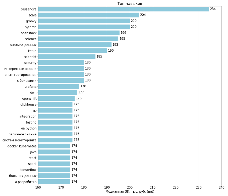
Top / Antitop skills
The charts were built for all 1994 uploaded vacancies. Salaries are indicated in 443 (22%) vacancies. For the calculation for each feature, vacancies were selected where this feature is present, and on their basis the median salary was calculated.

Job classification
Clustering could be made much easier without resorting to complex mathematical models: to compile the top names of vacancies, and divide them into groups. Next, analyze each group for top n-grams and average salaries. There is no need to highlight features and assign weights to them.
This approach would work well (to some extent) for a "Python" query. But for the request "1C Programmer" this approach will not work, because for 1C programmers in the names of vacancies, 1C configurations or applied areas are rarely indicated. And there are many areas where 1C is used: accounting, salary calculation, tax calculation, cost calculation at manufacturing enterprises, warehouse accounting, budgeting, ERP systems, retail, management accounting, etc.
For myself, I see two tasks for analyzing vacancies:
- Understand where a programming language that I know little about is used (as in this article).
- Filter new posted jobs.
Clustering is suitable for solving the first problem, for solving the second one - various classifiers, random forests, decision trees, neural networks. Nevertheless, I wanted to evaluate the suitability of the chosen model for the job classification problem.
If you use the predict () method built into sklearn.mixture.GaussianMixture , then nothing good happens. He attributes most of the vacancies to large clusters, and two of the first three clusters are uninformative. I used a different approach:
- We take the vacancy that we want to classify. We vectorize it and get a point in our space.
- We calculate the distance from this point to all clusters. Under the distance between a point and a cluster, I took the average distance from this point to all points in the cluster.
- The cluster with the smallest distance is the predicted class for the selected vacancy. The distance to the cluster indicates the reliability of such a prediction.
- To increase the accuracy of the model, I chose 0.87 as the threshold distance, i.e. if the distance to the nearest cluster is greater than 0.87, then the model does not classify the vacancy.
To evaluate the model, 30 vacancies were randomly selected from the test set. In the verdict column:
N / a: the model did not classify the job (distance> 0.87)
+: correct classification
-: incorrect classification
| Job vacancy | Nearest cluster | Distance | Verdict |
| 37637989 | Linux / DevOps Engineer | 0.9464 | N / a |
| 37833719 | C ++ Developer | 0.8772 | N / a |
| 38324558 | Data Engineer | 0.8056 | + |
| 38517047 | C ++ Developer | 0.8652 | + |
| 39053305 | Trash | 0.9914 | N / a |
| 39210270 | Data Engineer | 0.8530 | + |
| 39349530 | Frontend Developer | 0.8593 | + |
| 39402677 | Data Engineer | 0.8396 | + |
| 39415267 | C ++ Developer | 0.8701 | N / a |
| 39734664 | Data Engineer | 0.8492 | + |
| 39770444 | Backend Developer | 0.8960 | N / a |
| 39770752 | Data scientist | 0.7826 | + |
| 39795880 | Data Analyst | 0.9202 | N / a |
| 39947735 | Python Developer | 0.8657 | + |
| 39954279 | Linux / DevOps Engineer | 0.8398 | - |
| 40008770 | DevOps Engineer | 0.8634 | - |
| 40015219 | C ++ Developer | 0.8405 | + |
| 40031023 | Python Developer | 0.7794 | + |
| 40072052 | Data Analyst | 0.9302 | N / a |
| 40112637 | Linux / DevOps Engineer | 0.8285 | + |
| 40164815 | Data Engineer | 0.8019 | + |
| 40186145 | Python Developer | 0.7865 | + |
| 40201231 | Data scientist | 0.7589 | + |
| 40211477 | DevOps Engineer | 0.8680 | + |
| 40224552 | Data scientist | 0.9473 | N / a |
| 40230011 | Linux / DevOps Engineer | 0.9298 | N / a |
| 40241704 | Trash 2 | 0.9093 | N / a |
| 40245997 | Data Analyst | 0.9800 | N / a |
| 40246898 | Data scientist | 0.9584 | N / a |
| 40267920 | Frontend Developer | 0.8664 | + |
Total: 12 vacancies have no result, 2 vacancies - erroneous classification, 16 vacancies - correct classification. Model completeness - 60%, model accuracy - 89%.
Weak sides
The first problem - let's take two vacancies:
Vacancy 1 - "Lead C ++ Programmer"
"Requirements:
- 5+ years of C ++ development experience.
- Knowledge of Python will be an additional plus. "
Vacancy 2 - "Lead Python Programmer"From the point of view of the model, these vacancies are identical. I tried to adjust the weights of the features by the order of their occurrence in the text. This did not lead to anything good.
"Requirements:
- 5+ years of Python development experience.
- Knowledge of C ++ will be an additional plus "
The second problem is that GMM clusters all the points in a set, like many clustering algorithms. Non-informative clusters are not a problem by themselves. But informative clusters also contain outliers. However, this can be easily solved by clearing the clusters, for example, by removing the most atypical points that have the greatest average distance to the rest of the cluster points.
Other methods
The cluster comparison page demonstrates the various clustering algorithms well. GMM is the only one that gave good results.
The rest of the algorithms either did not work or gave very modest results.
Of those implemented by me, good results were in two cases:
- Points with a high density were selected in some neighborhood, located at a distant distance from each other. The points became the centers of the clusters. Then, on the basis of the centers, the process of cluster formation began - the joining of neighboring points.
- Agglomerative clustering is an iterative merging of points and clusters. The scikit-learn library presents this kind of clustering, but it does not work well. In my implementation, I changed the join matrix after each iteration of the merge. The process stopped when some boundary parameters were reached - in fact, dendrograms do not help to understand the merging process if 1500 elements are clustered.
Conclusion
The research I did gave me the answers to all the questions at the beginning of the article. I got hands-on experience with clustering while implementing variations of known algorithms. I really hope that the article will motivate the reader to carry out his analytical research, and will somehow help in this exciting lesson.