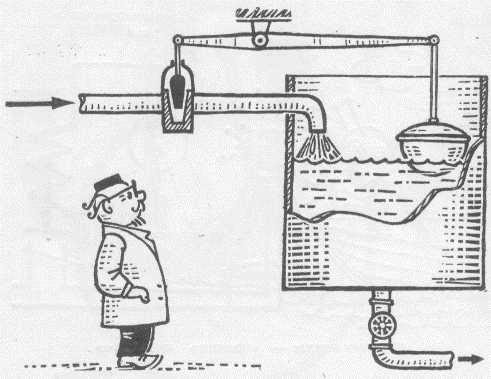
It is two-position because it has 2 positions: open (on) and closed (off), in the English-language literature on-off. There are also three or more positional regulators, that is, the water replenishment valve is open or closed to the main positions, and the “slightly open” position is added. After draining the water in the toilet, the float goes down, opening the valve completely and the water enters the tank at full pressure, but closer to reaching the set level, the float rises, closing the valve and reducing the flow of water. And as soon as the current water level (in English PV - Process Value - Current value ) rises to the set (in English SP - Set Point - Setpoint), the valve closes and the water level stops rising. In the described case, the regulator is even more similar to the proportional one - the regulating action decreases with decreasing mismatch (error), that is, the difference between the set level and the current level.
By slightly opening the lower pipe to drain the water, it will be possible to achieve such a state when the valve is fully open, and the water level does not decrease (that is, the inflow of water becomes equal to the source) - the system enters a state of equilibrium. But the problem is that this state is very precarious - any external disturbance can break this equilibrium - let's say we can scoop up a certain amount of water from the tank, and then it may happen that all the water will then flow out of the tank (due to the pressure change), or the replenishment pipe will become clogged and the flow will decrease, or the float will break and the water will overflow. This is the complexity of building control systems - real systems are quite complex and have many characteristics that must be taken into account.There is such a characteristic as the inertia of the system - if you turn off the heated stove, then it will remain hot for quite a long time, which is why more complex regulators are used to control the temperature, namelyPID - Proportional Integral Differential . Each of the components has its own characteristics - they all behave differently under different conditions, but when used together, they allow achieving fairly clear regulation. All these systems are calculated according to formulas, but in this case it is just important to understand how the system will behave when the PID controller coefficients change: with an increase in the proportional link, the initial impact increases and thus the system will be able to quickly achieve the required parameters. But if you overdo it, then overshoot may appear, which can be even worse than the low speed of the system.
During the existence of TAU, mathematical descriptions of many processes were found and now we can predict how the system will behave under certain circumstances. There are many simulation programs where you can set system parameters, set controller parameters and roughly see what will come of it. Walking around the Internet, I came across an Excel site for engineers, and there are several simulators of regulators, thanks to which you can look at the change in the process when changing the control factors. The easiest to repeat was, of course, the ON-OFF control., that is, in Russian, a two-position regulator. Let me remind you the principle of operation: if the current process value (Process value = PV) is the temperature, for example, below the setpoint (SP), then the regulator turns on (OP) - the heating elements are started at full power. As soon as the temperature reaches the set point, the regulator turns off the voltage supply to the heating elements.
Making a JavaScript simulator
To build a chart, I will use the ZingChart library - it turned out to be quite simple and easy to use. There are many examples in the documentation for which you can build anything at all. The plotting principle is quite simple - there is an array of values that are automatically placed on the graph in order, and thus a continuous process graph appears from a couple of hundred points. By the way, in the original in Excel, everything is done in the same way - 300 values are generated and a graph is built.
Actually, it is the generation of values that is the most difficult, namely the difficulty of correctly describing a process that correctly reacts to our control actions - turning on the heating elements - the temperature rises, turning off - falls, plus the inertia of the system must be put here. In addition, the heating environment can be different and some media heat up and cool down faster, and some vice versa, and if we adjust the level, then with the same flow from above, the level will rise higher in the tank where the bottom area is smaller. All this I lead to the fact that the process will also depend on the transmission (gain). In the original, a delay parameter was also introduced into the process (well, like the system does not immediately respond to the control signal), but I decided to abandon it - two are enough. But I added a change in the setting,although in fact it turned out that the setpoint can change from zero to 100, over 100 the process starts to behave differently, and apparently the reason is that the process formula is universal and does not describe a particular case. In general, let's start:
We create 5 fields for entering parameters, we put all this in a table, which we paint in a nice color above in css and place it in the center:
<table align="center" oninput="setvalues ();">
	<tr>
	<td>
Process parameters <br>
Gain: <input id="gain" type="number" value ="1" ><br>
Time Constant: <input id="time" type="number" value ="100" ><br>
	</td>
	<td>
Control parameters <br>
SetPoint(0-100): <input id="sp" type="number" value ="50"><br>
Hysteresis: <input id="hyst" type="number" value ="1">%<br>
	</td>
	<td>
Plot parameters <br>
Points: <input id="points" type="number" value ="200"><br>
	</td>
	</tr>
</table>
As you can see, each time the value of the fields inside the table changes, the setvalues () function will be called. In it, we read data from each field into special variables.
	let gain = document.getElementById('gain').value;
	let time = document.getElementById('time').value;
	let sp = document.getElementById('sp').value;
	let points = document.getElementById('points').value;
	let hyst = document.getElementById('hyst').value;
As already mentioned, to build a graph, you need arrays with data on the basis of which the graph will be built, so we create a bunch of arrays:
let pv = []; //
let pv100 = []; //   *100
let op = []; //   1 , 0
let pvp = 0; //
let low = sp-sp*hyst/100;//
let high = +sp+(sp*hyst/100); //
let st=true; //
Let me explain a little about hysteresis. The situation is this: when the temperature reaches the set value, the heating elements are turned off and immediately (in fact, not immediately, because there is inertia) the cooling process begins. And having cooled down by one degree or even a certain fraction of a degree - the system understands that it has already gone beyond the scope of the task again and it is necessary to turn on the heating elements again. In this mode, the heating elements will turn on and off very often, maybe even something that several times per minute - for equipment such a mode is not very good, and therefore, in order to exclude such fluctuations, a so-called hysteresis is introduced - deadband - a deadband - say 1 degree higher and below the setpoint, we will not react, and then the number of switchings can be significantly reduced. Therefore, the variable low is the lower limit of the setpoint, and the variable high is the upper one.The st variable keeps track of reaching the top level and allows the process to fall to the bottom. The logic of the whole process is in a loop:
	for (var i=0;i<points;i++) {
		if (pvp<=(low/100)) {
			st=true;
			op[i]=1;
			}//
		else if (pvp<=(high/100)&& st) op[i] = 1;
		else { st=false; op[i]=0;}

		let a = Math.pow(2.71828182845904, -1/time);
		let b = gain*(1 -a);
		pv[i] = op[i]*b+pvp*a;
		pv100[i] = pv[i]*100;
		pvp = pv[i];
	}
As a result, we get an array with a given number of points, which we send to the charting script.
scaleX: {
 	zooming: true
  },
      series: [
		{ values: op , text: 'OP' },
        { values: pv100 , text: 'PV'}
      ]
    };
Full code under the spoiler
<!DOCTYPE html>
<html>

<head>
  <meta charset="utf-8">
  <title></title>

  <script src="https://cdn.zingchart.com/zingchart.min.js"></script>
  <style>
    html,
    body,
    #myChart {
      width: 100%;
      height: 100%;
    }
	input {
	width: 25%;
	text-align:center;
	}
	td {

	background-color: peachpuff;
	text-align: center;
	}
  </style>
</head>
<body>
<table align="center" oninput="setvalues ();">
	<tr>
	<td>
Process parameters <br>
Gain: <input id="gain" type="number" value ="1" ><br>
Time Constant: <input id="time" type="number" value ="100" ><br>
	</td>
	<td>
Control parameters <br>
SetPoint(0-100): <input id="sp" type="number" value ="50"><br>
Hysteresis: <input id="hyst" type="number" value ="2">%<br>
	</td>
	<td>
Plot parameters <br>
Points: <input id="points" type="number" value ="250"><br>
Animation: <input type="checkbox" id="animation">
	</td>
	</tr>
</table>

<script>

setTimeout('setvalues ()', 0);

function setvalues (){

	let gain = document.getElementById('gain').value;
	let time = document.getElementById('time').value;
	let sp = document.getElementById('sp').value;
	let points = document.getElementById('points').value;
	let hyst = document.getElementById('hyst').value;
	let anim = document.getElementById('animation').checked ? +1 : 0;
	let pv = []; //
	let pv100 = []; //   *100
	let op = []; //   1 , 0
	let pvp = 0; //
	let low = sp-sp*hyst/100; //
	let high = +sp+(sp*hyst/100); //
	let st=true; //
	for (var i=0;i<points;i++) {
		if (pvp<=(low/100)) {
			st=true;
			op[i]=1;
			}
		else if (pvp<=(high/100)&& st) op[i] = 1;
		else { st=false; op[i]=0;}

		let a = Math.pow(2.71828182845904, -1/time);
		let b = gain*(1 -a);
		pv[i] = op[i]*b+pvp*a;
		pv100[i] = pv[i]*100;
		pvp = pv[i];
	}

	ZC.LICENSE = ["569d52cefae586f634c54f86dc99e6a9", "b55b025e438fa8a98e32482b5f768ff5"];
    var myConfig = {
    type: "line",
    "plot": {
		"animation": {
          "effect": anim,
          "sequence": 2,
          "speed": 200,
        }
		},
	legend: {
    layout: "1x2", //row x column
    x: "20%",
    y: "5%",
	},
 	crosshairX:{
 	  plotLabel:{
 	    text: "%v"
 	  }
 	},
      "scale-y": {
    item: {
      fontColor: "#7CA82B"
    },
    markers: [
	 {
        type: "area",
        range: [low, high],
        backgroundColor: "#d89108",
        alpha: 0.7
      },
	{
        type: "line",
        range: [sp],
        lineColor: "#7CA82B",
        lineWidth: 2,
		  label: { //define label within marker
          text: "SP = "+sp,
          backgroundColor: "white",
          alpha: 0.7,
          textAlpha: 1,
          offsetX: 60,
          offsetY: -5
        }
      }]
	},
	scaleX: {
		zooming: true
	},
	  'scale-y-2': {
	  values: "0:1"
	},
      series: [
		{ scales: "scale-x,scale-y-2", values: op , 'legend-text': 'OP' },
        { values: pv100 , text: 'PV'}
      ]
    };

    zingchart.render({
      id: 'myChart',
      data: myConfig,
      height: "90%",
      width: "100%"
    });
}


</script>
  <div id='myChart'></div>
</body>
</html>
Well, since the simulator is ready, it's time to check out how it works. You can test here the same code but on the github: on-off control simulator
Standard setting: amplifying link 1, time constant 100 seconds, hysteresis 2%

Now if you set a larger setting, for example 92, then suddenly the process slows down a lot, although the setting is 50 it gains in the same 71 seconds, but only then the curve begins to approach the task more slowly exponentially, and reaches the setpoint in only 278 seconds, which is why it was necessary to expand the plotting range to 300 points

This example is very indicative, translating the situation to a model with temperature, we can conclude that there is not enough heater power: the heater is 100% loaded, but the temperature stops rising after a certain moment. There may be several solutions: to put a second heating element of the same, or to apply voltage to it 2 times more (but this can damage the heating element), or to put a heater with 2 times more power, or to pour a more heat-conducting liquid into the system when it comes to heating liquids. Interestingly enough, if you need to maintain the temperature in the region of 95-100 degrees, then you don't even need to put the regulator - put such a low-power heater, turn it on to its fullest and that's it - after 300 seconds (conditional 300 seconds) you can get the desired 100 degrees.The problem with such a system is that if you open a window in winter at minus 40, then the temperature will immediately drop and quite significantly, and the speed of such a system is very low.
Let's increase the gain section by 2 times - it's like installing a second heating element of the same type, or adding another pipe to replenish the tank.

The graph turned out to be also quite indicative - the temperature reached 51 degrees actually reached 2 times faster, but reached 92 degrees 4 times faster. I do not know how close such a simulator is to real processes, but since the dependence specified in it is exponential, this is a completely expected behavior of the system, but I cannot even imagine explaining from the perspective of adding a second pipe and increasing the filling rate by 4 times. The response of a linear function would be more predictable to an increase in the coefficient, but real systems in life are rarely linear.