
What does the data look like?
First, let's look at the available test and training data (data from the Toxic comment classification challenge on the kaggle.com platform). In the training data, in contrast to the test data, there are labels for classification:
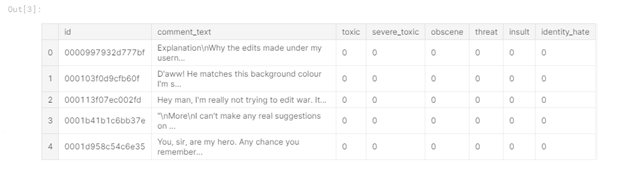
Figure 1 - Train data head
From the table you can see that we have 6 label columns in the training data ("toxic", "severe_toxic", "obscene", "threat" , "Insult", "identity_hate"), where the value "1" indicates that the comment belongs to the class, there is also a column "comment_text" containing the comment and a column "id" - the comment identifier.
Test data does not contain class labels, as it is used to send the solution:

Figure 2 - Test data head
Feature extraction
The next step is to extract features from comments and conduct exploratory data analysis (EDA). First, let's look at the distribution of comment types in the training dataset. For this, a new column "toxic_type" was created, containing all the classes to which the comment belonged:

Figure 3 - Top-10 types of toxic comments
From the table you can see that the prevailing type is the absence of any class labels, and many comments belong to more than one class.
Let's also see how the number of types is distributed for each comment:

Figure 4 - Number of types encountered
Note that the prevailing situation is when a comment is characterized by only one type of toxicity, and quite often the comment is characterized by three types of toxicity, and less often the comment is attributed to all types.
Now let's move on to the stage of extracting features from text, which is often called features extraction. I extracted the following attributes:
Length of the comment. I guess the angry comments are likely to be short;
Uppercase. In aggressive-emotional comments, it is possible that the upper case will be more common in words;
Emoticons. When writing a toxic comment, positively colored emoticons (:), etc.) are unlikely to be used, also consider the presence of sad emoticons (:(, etc.);
Punctuation. Probably, the authors of negative comments do not adhere to the rules of punctuation, to a greater extent they use "!";
The number of third-party characters. Some people often use the @, $, etc. symbols when writing offensive words.
Features are added as follows:
train_data[‘total_length’] = train_data[‘comment_text’].apply(len)
train_data[‘uppercase’] = train_data[‘comment_text’].apply(lambda comment: sum(1 for c in comment if c.isupper()))
train_data[‘exclamation_punction’] = train_data[‘comment_text’].apply(lambda comment: comment.count(‘!’))
train_data[‘num_punctuation’] = train_data[‘comment_text’].apply(lambda comment: comment.count(w) for w in ‘.,;:?’))
train_data[‘num_symbols’] = train_data[‘comment_text’].apply(lambda comment: sum(comment.count(w) for w in ‘*&$%’))
train_data[‘num_words’] = train_data[‘comment_text’].apply(lambda comment: len(comment.split()))
train_data[‘num_happy_smilies’] = train_data[‘comment_text’].apply(lambda comment: sum(comment.count(w) for w in (‘:-)’, ‘:)’, ‘;)’, ‘;-)’)))
train_data[‘num_sad_smilies’] = train_data[‘comment_text’].apply(lambda comment: sum(comment.count(w) for w in (‘:-(’, ‘:(’, ‘;(’, ‘;-(’)))
Exploratory data analysis
Now let's explore the data using the features we just got. First of all, let's look at the correlation of features with each other, the correlation between features and class labels, the correlation between class labels:

Figure 5 - Correlation
Correlation indicates the presence of a linear relationship between the features. The closer the value of the correlation in modulus is to 1, the more pronounced the linear dependence between the elements.
For example, you can see that the number of words and the length of the text are strongly correlated with each other (value 0.99), which means that some feature can be removed from them, I removed the number of words. We can also draw several more conclusions: there is practically no correlation between the selected features and class labels, the least correlated feature is the number of characters, and the length of the text correlates with the number of punctuation characters and the number of characters converted to uppercase.
Next, we will build several visualizations for a more detailed understanding of the influence of features on the class label. First, let's see how the comment lengths are distributed:

Figure 6 - Distribution of comment lengths (the graph is interactive, but here is a screenshot)
As expected, comments that have not been categorized (i.e. normal) are much longer in length than tagged comments. Of the negative comments, the shortest are threats, and the longest are toxic.
Now let's examine comments in terms of punctuation. We will build graphical representations for average values to make the graphs more interpretable:

Figure 7 - Average punctuation values (the graph is interactive, but here is a screenshot)
From the figure you can see that we got three clusters.
The first one is normal comments, they are characterized by observance of punctuation rules (placement of punctuation marks, ":", for example) and a small number of exclamation marks.
The second consists of threats (threat) and very toxic comments (severe toxic), for such a group is characterized by abundant use of exclamation marks and other punctuation marks are used at the middle level.
The third cluster - toxic (toxic), obscene (obscene), insults (insult) and hateful towards a certain person (identity hate) have a small number of both punctuation marks and exclamation points.
Let's add a third axis for clarity - upper case:

Figure 8 -Three-dimensional image (interactive, but here's a screenshot)
Here we see a similar situation - three clusters are highlighted. Also note that the distance between the elements of the second cluster is greater than the distance between the elements of the third cluster. This can be seen in the 2D graph as well:

Figure 9 - Upper case and punctuation (interactive, here's a screenshot)
Now let's look at the types of comments in the context of upper case / the number of third-party characters:

Figure 10 - Upper case and the number of third-party characters (interactive, here's a screenshot)
As you can see, very toxic comments are clearly highlighted - they have a large number of uppercase characters and many third-party characters. Also, third-party symbols are actively used by the authors of comments hateful to some person.
Thus, highlighting new features and visualizing them allows for better interpretation of the available data, and the above constructed visualizations can be summarized as follows:
Highly toxic comments are separated from the rest;
Normal comments also stand out;
Toxic, obscene and offensive comments are very close to each other in terms of the characteristics considered.
Using the DataFrameMapper to Combine Text and Numeric Features
Now, let's look at how you can use text and numeric features together in Logistic regression.
First, you need to choose a model to represent the text in a form suitable for machine learning algorithms. I used the tf-idf model, as it is able to highlight specific words and make frequent words less significant (for example, prepositions):
tvec = TfidfVectorizer(
sublinear_tf=True,
strip_accents=’unicode’,
analyzer=’word’,
token_pattern=r’\w{1,}’,
stop_words=’english’,
ngram_range=(1, 1),
max_features=10000
)
So, if we want to work with the dataframe provided by the Pandas library and the machine learning algorithms of the Sklearn library, we can use the Sklearn-pandas module, which serves as a kind of binder between dataframe and Sklearn methods.
mapper = DataFrameMapper([
			([‘uppercase’], StandardScaler()),
			([‘exclamation_punctuation’], StandardScaler()),
			([‘num_punctuation’], StandardScaler()),
			([‘num_symbols’], StandardScaler()),
			([‘num_happy_smilies’], StandardScaler()),
			([‘num_sad_smilies’], StandardScaler()),
			([‘total_length’], StandardScaler())
		], df_out=True)
First you need to create a DataFrameMapper as shown above, it should contain the names of the columns that have numeric features. Next, we create a matrix of features, which we will then transfer to Logistic regression for training:
x_train = np.round(mapper.fit_transform(numeric_features_train.copy()), 2).values
x_train_features = sparse.hstack((csr_matrix(x_train), train_texts))
A similar sequence of actions is also performed on the test data set.
Computational experiment
To carry out multi-label classification, we will build a loop that will go through all categories and evaluate the quality of the classification by cross-validation with the parameters cv = 3 and scoring = 'roc_auc':
scores = []
class_names = [‘toxic’, ‘severe_toxic’, ‘obscene’, ‘threat’, ‘identity_hate’]
for class_name in class_names:
	train_target = train_data[class_name]
	classifier = LogisticRegression(C=0.1, solver= ‘sag’)
	cv_score = np.mean(cross_val_score(classifier, x_train_features, train_target, cv=3, scoring= ‘auc_roc’))
	scores.append(cv_score)
	print(‘CV score for class {} is {}’.format(class_name, cv_score))
	classifier.fit(train_features, train_target)

print(‘Total CV score is {}’.format(np.mean(scores)))</source
<b> :</b>

<img src="https://habrastorage.org/webt/kt/a4/v6/kta4v6sqnr-tar_auhd6bxzo4dw.png" />
<i> 11 —  </i>

      ,       ,  , ,       ,   .  ,    ,       ,      .    - ,   “toxic”, ,  ,       (  3).         , ,          ,        .