Real systems can only be considered linear over a limited range of loads. The real world around us is not linear (Fig. 1). Nonlinearity is a violation of the principle of superposition in a certain phenomenon (mechanical system): the result of the action of the sum of factors is not equal to the sum of the results from individual factors. However, for various reasons, including the lack of the necessary knowledge, modeling skills, and the necessary software, engineers often solve problems only in linear formulations. Even when the linear approach gives very large errors. Accurate modeling of system behavior often requires nonlinear analysis.
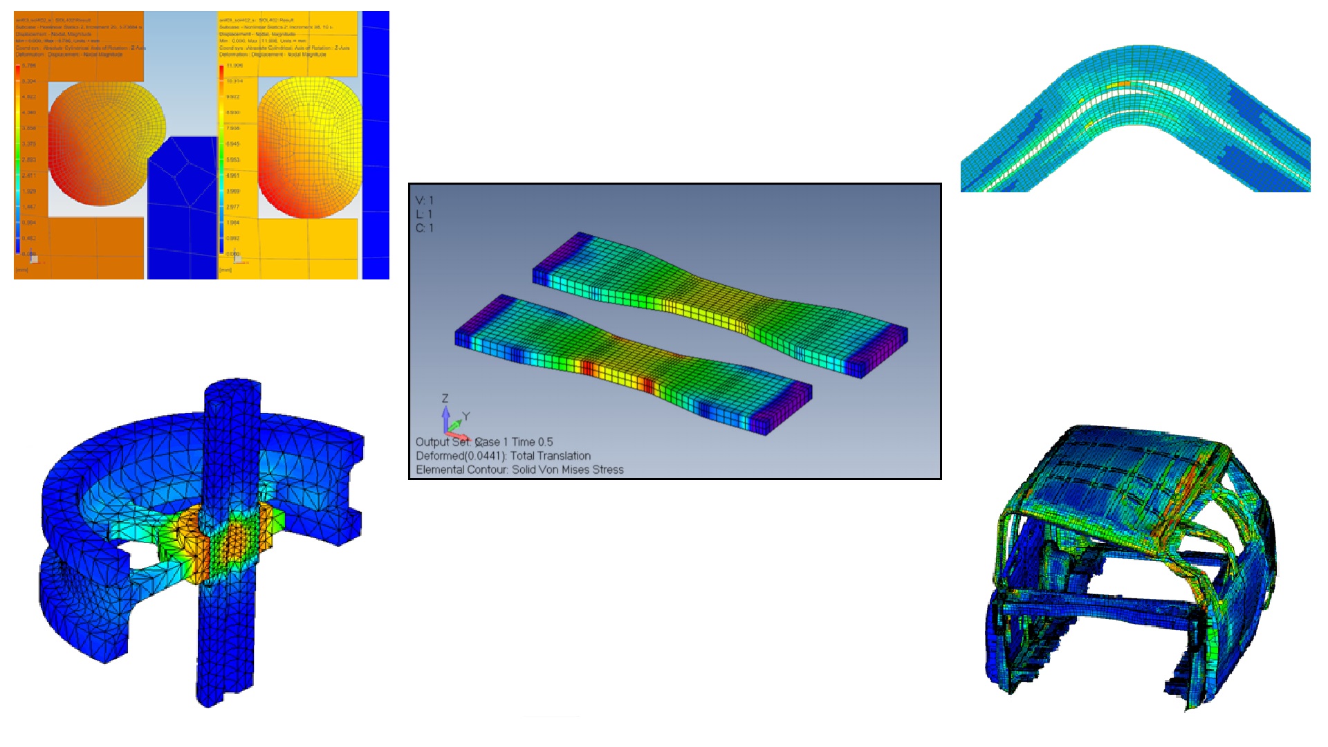
Figure: 1
Introduction
A couple of months ago I published an article “Just About Nonlinear Finite Element Analysis. An example of a bracket . " In it, I tried to explain in an accessible way the minimum amount of terms and theory necessary for the conscious conduct of nonlinear static analysis, I analyzed in detail the algorithm for solving a simple nonlinear problem. I will not repeat myself, I will remind you of a few basic provisions - and we will proceed to an overview of more complex phenomena, problems of mechanics and the tools necessary to solve these nonlinear problems.
Linear assumptions are often valid, but non-linear calculations are increasingly required in product development today. To reduce the amount of experimental development, users need models of higher accuracy: geometric models are refined, the accuracy of physical models is increased. This means that non-linear effects such as contacts, large deformations and material properties are taken into account. The nonlinearity of the problem may be due to the need to take into account the history of the loading of the structure - that is, the decomposition of the problem into components of the impact and the subsequent combination of the results is impossible. If these effects are not taken into account, decisions may be inaccurate, leading to incorrect conclusions. Alternatively, products may be designed with a very large margin of safety and therefore become too expensive.
We have one classical physics and mathematics, but different computational complexes use different sets of algorithms and tools to solve problems by the finite element method. In this article, I will discuss the tools available in the Femap pre-post processor with NX Nastran solver, which has been proven reliable, accurate and fast over 35 years. For solving the most complex nonlinear problems, including if it is necessary to take into account the load history of a structure, the Multistep Nonlinear (SOL401 / SOL402) multistep nonlinear solution module is suitable.
Contacts and the use of sub-cases
Within a single multi-step solution, you can change the contact conditions of surfaces using sub-cases . Sub-cases are separate solutions from which you can add a general solution with a complex history of load application, changes in boundary conditions. For example, when modeling an assembly, you can add or remove contacts in sequence.
Friction can be taken into account in the contact settings, and the coefficient of friction can be constant or vary with speed, temperature and time. Parts that are in contact are usually considered deformable. But if one part is much more rigid than the other, it is worth considering it as rigid in order to simplify the task without significant errors. It also allows the forced movement of a rigid body to be applied to a rigid part as a load.
In fig. 2 shows a model in which the rubber O-ring is defined by a hyperelastic material. The simulation computes the stresses and displacements in the rubber O-ring used to seal the bonnet fitted to the cylinder. In order to improve efficiency, the model is built using axial symmetry. The visible circle is the cross section of the O-ring. The unstressed seal ring is smaller than the cylinder diameter, so the initial position of the seal ring indicates that the seal ring and cylinder overlap. In the first simulation step, overlap is compensated for contact detection, that is, the O-ring is radially stretched. Then the cap is lowered and the O-ring deforms on contact with the cylinder wall.Thus, a seal is formed.

Figure: 2
Geometric imperfections of the finite element mesh can be corrected by adjusting clearance and interference tolerances or by smoothing the edges. When convergence difficulties arise, there are many options for solving this problem. For example, the Normal Regularization option is useful when the contact conditions include soft materials such as rubber. Tangential regularization avoids discontinuities in frictional forces. In addition, local stiffness and damping at the contact is user controlled, which can also be used to improve convergence. The following results can be analyzed in the postprocessor: contact pressure, normal distance, slip, contact forces.
There are many contact applications including bolting, drop simulation, and interference fit. You can model bolted connections using 1D finite elements (beams, bars), 2D (planar elements), or 3D elements. Preloading can be done with multiple sub-cases - for example, if you want to simulate a bolt tightening sequence. Pretensioning sub-cases can be implemented not only first in a row, but also in any sequence. When analyzing other sub-cases, the calculated prestresses are retained, but the actual bolt load may change with further application of loads. Users can analyze normal stress, shear stress, bolt moments - throughout the solution.
In fig. 3 depicts a model that analyzes the following assembly / loading / unloading sequence: tighten bolt # 1, tighten bolt # 4, tighten bolt # 2, tighten bolt # 3, apply service load, remove load, release.

Figure: 3
Large displacements (deformations) and analysis after buckling
Large linear and angular displacements are fundamental nonlinear effects (Figure 4). They take into account the change in the position of the load as the system deforms. There is also the effect of changing the rigidity of the product from the load. The buckling solution is a nonlinear solution with large strain effects enabled.
The load causes a loss in the rigidity of the product, leading to subsequent large deformations with small changes in the load. Efficient algorithms exist to analyze the system after the critical buckling load has been exceeded.

Figure: 4
Analysis after bucklingIs a special type of static subcase in Femap. In standard quasi-static analysis, loads are increased according to a user-defined law. However, some products are unstable due to their shape after reaching a certain load level. Such products abruptly lose their rigidity in a certain range of loads. To solve this kind of problems, the "arc length" algorithm should be used - it is used to solve the problems of unstable bending, loss of stability. The solution allows not only to determine the critical load of buckling in bending, but also to analyze how the structure will behave after it becomes unstable. Instead of changing the loads based on time increments, the algorithm automatically changes the load increments in proportion to displacement, not time.
The initial imperfections of the shape have a great influence in the problems of buckling. Shape imperfections can be accounted for as distortions in the geometry / mesh, which can be used to account for imperfections in the manufacturing process. The user can simulate the places of deliberate bending or simulate the damage received during operation.
Physical nonlinearity (nonlinearity of material properties). Plasticity, hyperelasticity, toughness, creep and composites
In traditional linear analysis, all materials are considered linear and elastic. Femap multistep nonlinear solver supports nonlinear properties along with isotropic, orthotropic, anisotropic behavior. Several other non-linear material behavior models are also supported, including plasticity, hyperelasticity, creep, and damage. Users who need to set unique material properties are given the option to optionally add their own material models.
Plastic Material Modelswith different settings are available for simulation. Users can define the stress-strain curve as bilinear or multilinear (Figure 5). Loading / unloading effects can be described using isotropic, kinematic or mixed hardening models. Stress-strain curves can also be supplemented with temperature dependence. Thus, materials, the dependence of the properties of which on temperature must be taken into account when solving the problem, can be adequately described.

Figure: 5
Hyperelastic materialsdue to their properties, they are widely used in various industries. They are independent of the strain rate. Such materials include rubber, foam, biological and polymer materials. They support very large deformations (more than 600%), are practically incompressible, and they can also be temperature dependent. Standard material models of Mooney-Rivlin, Ogden with Mullins effect and foam models are available. In fig. 6 shows a model of the gear shift handle cover. The shroud material is specified as a hyperelastic rubber material using the Mooney-Rivlin model. The surfaces of the casing are tuned for self-contact.

Figure: 6
Viscoelastic materials are elastic materials with the ability to dissipate mechanical energy due to the influence of viscosity.
Elastic materials such as rubber stretch instantly and quickly return to their original state when the load is removed. Viscosity (internal friction) is the property of a body to resist the movement of one part of it relative to another. Femap supports viscoelastic materials with Kelvin and Prony series formulations. The Kelvin model reflects the phenomenon of elastic aftereffect, which is a change in elastic deformation over time, when it either constantly increases to a certain limit after the application of the load, or gradually decreases after it is removed (Fig. 7). When the tension is released, the material gradually relaxes to an undeformed stage. The Kelvin model is used for organic polymers, rubber, wood at low stress.

Figure: 7
Creep type deformationsoccur over time without any change in load. Deformation during creep, as in plasticity, is irreversible (inelastic), the behavior of the material during creep is incompressible.
Many materials, especially under high temperature conditions, can undergo creep deformations. Femap uses the standard Bailey-Norton creep model and allows you to define temperature dependencies for the governing factors.
In most materials, under the action of a constant load, three stages of creep are distinguished (Fig. 8). In the first stage, the strain rate decreases with time. This phenomenon is observed for a short period of time. The second stage, which is longer, is characterized by a constant strain rate. At the third stage, the deformation rate rapidly increases until the material is completely destroyed (sample rupture).

Figure: 8 The
Femap multistep nonlinear solver can model the nonlinear behavior of composites as a result of interlayer or interlayer fracture (Figure 9).
In the case of intra-layer destruction, individual layers weaken and lose their rigidity when a certain load level is exceeded. The solver monitors the stiffness of each layer in the assembly and updates the stiffness of the feature as the layers become more damaged. In extreme cases, a complete loss of stiffness in the element can occur. Intra-layer fractures (for a unidirectional or woven layer) are of various types: fiber destruction, matrix destruction, destruction of bonds between the matrix and fibers.
With interlayer destruction, the bond between the layers of the product can weaken and lose rigidity. Femap uses binders to model this behavior. The simulation shows areas where bond is lost and layers can be detached.

Figure: nine
Load history accounting. Multi-step solutions using sub-cases
The state of the structure in some cases depends on the sequence of application of loads, that is, the nonlinearity of the problem may be due to the need to take into account the history of loading of the structure. There are problems in which it is sufficient to take into account the initial stress-strain state (often for nonlinearities associated with the behavior of the material). But sometimes it is necessary to take into account a complex loading history, consisting of several sub-cases with varying force factors and boundary conditions. The boundary conditions can change when the contact areas change.
An important feature of the Femap multistep nonlinear solver is that it can support multiple sub-cases and execute different solutions - such as static, dynamic, modal in separate sub-cases within one solution. In addition to changing the analysis type in sub-cases, you can also change parameter settings and boundary conditions. This gives users great flexibility in customizing their solutions. Here is a typical scenario using sub-cases: each sub-case begins with the conditions in which the previous sub-case ended. This subcase is called sequential. But the user can also start the solution again and not in a sequential subcase.
In fig. 10 shows an example of modeling three components of an aircraft engine: two flanges and a hub are bolted together in several stages. For an effective solution, a symmetrical sector of the model is used. In the first step, the deviations from the mold for one flange and hub are analyzed. On the second, two bolts are tightened to connect the flange and hub. The third examines the pressing of the second flange. On the fourth, two more bolts are tightened to connect the second flange to the hub. Then, in the fifth step, the load from the high-speed rotation of the fully connected parts is analyzed. The last step is modal analysis - it is used to predict vibration stresses. This complete set of six steps can be performed in a single analysis,which allows obtaining a rich set of data for understanding the stress-strain state of the engine.

Figure: 10
In addition to static sub-cases, dynamic (transient) ones are supported. This type of subcase can start a solution or follow static subcase (Figure 11). When running the solution, initial conditions in the form of displacement or velocity can be applied. For example, to simulate a fall, it is rational to start the solution from a point immediately before the impact and set the initial velocity equal to the impact velocity. If dynamic analysis follows static or other dynamic analysis, then deviations, velocities, accelerations at the beginning of the subcase will be the same as at the end of the previous subcase.
In a dynamic subcase, the generated inertia forces, damping, stiffness matrix and forces are balanced by the applied loads. Inertia forces can be disabled during transient analysis. This is very useful for speeding up the solution and going to a steady state.

Figure: eleven
Dynamic analysis and modeling of kinematic links
Fall simulations are often performed on electronic devices to understand how well they will survive impact with the ground. In fig. 12 shows the shock process that occurs when a thermal imaging camera falls. The polycarbonate housing material is modeled as an elastoplastic material, while the internal PCB and electronic components are modeled as linear elastic materials. The dynamic analysis starts from the point of contact of the thermal imager with the ground. The camera is given an initial velocity corresponding to the height from which it was dropped (in this case, it is 1 meter). The camera quickly hits the ground and bounces. Stresses and deformations of the hull and sides are analyzed.

Figure: 12
Femap supports the use of kinematic constraintsto connect different parts of the assembly. Basic hinge types are supported such as cylindrical, spherical, rigid and flexible guides.
In fig. 13 depicts the process of deploying solar panels on a satellite connected by a cylindrical hinge. With this model, vibrations and stress levels can be estimated.

Figure: 13
Conclusion
The main quality criteria for evaluating the design model and the results obtained have always been and will be comparison with field experiments and analytical solutions. Non-linear models are no exception to the rule. Femap developers from Siemens validate nonlinear formulations using NAFEMS (International Association for Analysis and Modeling Engineering) tests and analytical solutions.
In addition to formulation checking, algorithms are regularly tested against a large library of test models to avoid bugs as improvements and extensions are added.
However, each engineer faces the question of the adequacy of the assumptions made, the correct use of available software tools and the multi-criteria assessment of the results obtained.
This article provides an overview of current nonlinear problems and tools for their solution. Of course, this information is not enough to start solving the above problems in practice. Therefore, I invite you to a free webinar "Femap and the capabilities of the module of multistep nonlinear solutions Multistep Nonlinear" , which will be held on November 19, 2020 at 12:00. In the second half of the webinar, I will solve the problem of stretching a metal sample, taking into account the plasticity and isotropic hardening of the material. You can read an overview of the capabilities of the Femap computational complex with NX Nastran here , and download a free trial version of Femap with NX Nastran here . Philip Titarenko, product manager for Femap

JSC Nanosoft
E-mail: titarenko@nanocad.ru
References
1. Femap with NX Nastran, Simcenter 3D Multistep nonlinear solvers: SOL401 / SOL402.Multistep Nonlinear (translated by F.V. Titarenko). Siemens.
2. NX Nastran Handbook of Nonlinear Analysis (Solutions 106 and 129). Siemens.