How do we know the algorithm works?
Before developing an algorithm, you need to think about how we will evaluate its performance. Let's say we wrote an algorithm, and it says that "this image has the following colors" - will his decision be correct? And what does that even mean - "correct"?
To solve this problem, we have chosen two important dimensions - the correct marking of the primary color and the correct number of colors. We set this as the distance CIEDE 2000 ( color difference formula ) between the foreground color predicted by our algorithm and our actual foreground color, and we also calculate the average absolute error in the number of colors. We made this choice for the following reasons:
- These parameters are easy to calculate.
- As the number of metrics increased, it would be more difficult to choose the “best” algorithm.
- By reducing the number of metrics, we may be missing an important difference between the two algorithms.
- In any case, most garments have one or two primary colors, and many of our processes rely on a primary color. Therefore, calculating the base color correctly is much more important than calculating the second or third color correctly.
What about "real" data? Our team of merchandisers provided us with labels, but our tools allow them to choose only the most common colors, such as "gray" or "blue" - they cannot be called an exact value. Such general definitions include quite a few different shades, so they cannot be used as real colors. We'll have to build our own dataset.
Some of you might already be thinking about services like Mechanical Turk. But we don't need to mark up too many images, so describing this task may be even harder than just completing it. In addition, creating a dataset helps you better understand it. We quickly bungled an HTML / Javascript application and randomly selected 1000 images, selected for each pixel that represents its primary color, and marked the number of colors we saw in the image. After that, it became easy to get two numbers evaluating the quality of our algorithm (distance to the main color CIEDE and the number of colors MAE).
Sometimes we checked the programs manually, running both algorithms on one image and displaying two lists of colors. We then manually rated 200 images, choosing which colors were recognized “best”. It is very important to work closely with the data in this way - not only to get the result (“Algorithm B worked better than Algorithm A in 70% of cases”), but also to understand what happens in each of the cases (“Algorithm B usually selects too many groups, but Algorithm A misses light colors ”).

Sweater and colors selected by two different algorithms
Our color extraction algorithm
Before processing the images, we convert them to the CIELAB (or just LAB) color space instead of the more common RGB. As a result, our three numbers will not represent the amount of red, green and blue. The points of the LAB space (L * a * b * would be more correct, but we will write LAB for simplicity) designate three different axes. L denotes luminance from black 0 to white 100. A and B denote color: A denotes a location in the range from -128 green to 127 red, and B from -128 blue to 127 yellow. The main advantage of this space is perceived uniformity. The distance or difference between two points in LAB space will be perceived the same, regardless of their location, if the Euclidean distance between them in space is also the same.
Naturally, the LAB has other problems: for example, we consider images on computer screens that use device-specific RGB space. Also, the LAB gamut is wider than that of RGB, that is, in LAB you can express colors that cannot be expressed through RGB. Therefore, the conversion from LAB to RGB cannot be two-sided - by converting a point in one direction and then in the opposite direction, you can get a different value. Theoretically, these shortcomings are present, but in practice the method still works.
By converting the image to LAB, we will get a set of pixels that can be viewed as points (L, A, B, X, Y). The remainder of the algorithm is concerned with grouping these points, in which the groups of the first stage use all five measurements, and the second one omits the X and Y measurements.
Grouping in space
We start with an image without pixel grouping that has undergone the color adjustments described in the previous article , compressed to 320x200 and converted to LAB.
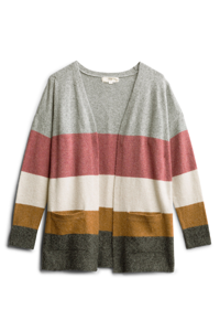
First, let's apply the Quickshift algorithm, which groups nearby pixels into “superpixels”.
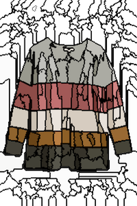
This already reduces our 60,000 pixel image to a few hundred superpixels, removing unnecessary complexity. You can simplify the situation even more by merging together nearby superpixels with a small color distance between them. To do this, we draw their regional proximity graph - a graph in which the nodes denoting two different superpixels are connected by an edge if their pixels touch.
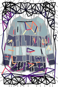
– (Regional Adjacency Graph, RAG) . , , , , . , , , , . – , .
The nodes of the graph are the superpixels we calculated, and the edges are the distance between them in the color space. The edge connecting two nearby superpixels with similar colors will have a low weight (dark lines), and the edge between superpixels with very different colors will have a high weight (bright lines, as well as the absence of lines - they were not drawn if their weight was more than 20). There are many ways to combine nearby superpixels, but a simple threshold of 10 was enough for us.
In our case, we managed to reduce 60,000 pixels to 100 areas, each of which contains pixels of the same color. This gives computational advantages: First, we know that a large superpixel of almost white color is the background and can be removed. We remove all superpixels with L> 99, and A and B in the range from -0.5 to 0.5. Second, we can greatly reduce the pixel count in the next step. We will not be able to reduce their number to 100, since we need to weigh the areas based on the number of pixels they contain. But we can easily remove 90% of the pixels from each group without losing too much detail and almost no distortion of the next grouping.
Grouping without using space
At this step, we have several thousand pixels with coordinates (L, A, B). There are many techniques that can group these pixels nicely. We chose the k-means method because it is fast, easy to understand, our data only has 3 dimensions, and the Euclidean distance in LAB space makes sense.
We weren't too clever and had a grouping with K = 8. If some group contains less than 3% of points, we try again, this time with K = 7, then 6, and so on. As a result, we have a list of 1 to 8 centers of grouping and the proportion of the number of points belonging to each of the centers. They are named by the colornamer algorithm described in the previous article.
Results and remaining problems
We achieved an average distance of 5.86 on the CIEDE 2000 scale between predicted and “real” color. It is rather difficult to correctly interpret this indicator. On the simple CIE76 distance metric, our average distance is 7.82. On this metric, a value of 2.3 represents a subtle difference. Therefore, we can say that our results, slightly over 3, indicate a subtle difference.
Also our MAE was 2.28 colors. But again, this is a secondary metric. Many algorithms described below reduce this error, but at the expense of increasing the color distance. It is much easier to ignore the 5th or 6th place false colors than to ignore the wrong 1st color.
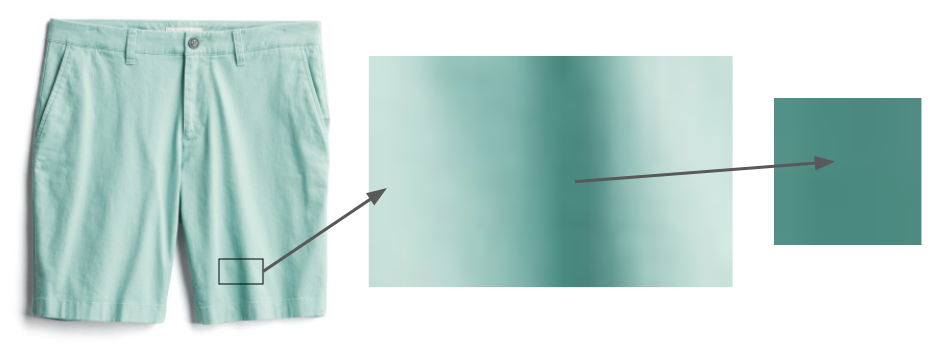
Even things that are clearly the same color, like these shorts, contain areas that appear much darker due
to shadows. The problem of shadows remains. The fabric cannot be laid perfectly evenly, therefore, part of the image will always remain in the shadow, and it will seem deceptively of a different color. The simplest approaches such as finding duplicate colors of the same shade and different brightness do not work, since the transition from “pixel without shadow” to “pixel in shadow” does not always work the same way. In the future, we hope to use more sophisticated techniques like DeshadowNet or automatic shadow detection .
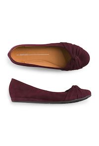
We only concentrated on the color of the clothes. Jewelry and shoes have their own problems: our photographs of jewelry are too small, and photographs of shoes often show the insides of them. In the example above, we would indicate the presence of burgundy and ocher in the photo, although only the first of them is important.
What else have we tried
This last algorithm seems pretty simple, but it wasn't easy to come up with! In this section, I will describe the options we have tried and learned from.
Background Removal
We have tried background removal algorithms - for example, the algorithm from Lyst . Informal evaluation showed that they did not work as accurately as simple removal of the white background. However, we plan to study it deeper as we process images that our photo studio did not work on.
Hashing pixels
Some color extraction libraries have chosen a simple solution to this problem: group pixels by hashing them into several sufficiently wide containers, and then return the average values of the LAB containers with the largest number of pixels. We tried out the Colorgram.py library; despite its simplicity, it works surprisingly well. In addition, it works quickly - no more than a second per image, while our algorithm spends tens of seconds per image. However, Colorgram.py had a larger average distance to the base color than our algorithm - mainly because its result is taken from the average distances to large containers. However, we sometimes use it for cases where speed is more important than accuracy.
Another superpixel splitting algorithm
We use the Quickshift algorithm to segment the image into superpixels, but there are several possible algorithms - for example, SLIC, Watershed and Felzenszwalb. In practice, Quickshift has shown the best results thanks to its work with small parts. For example, SLIC has a problem with things like stripes taking up a lot of space in the picture. Here are the indicative results of the SLIC algorithm with different settings:
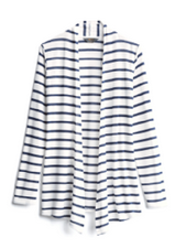
Original image
compactness = 1

compactness = 10

compactness = 100
To work with our data, Quickshift has one theoretical advantage: it does not require continuous superpixel communication. The researchers noted that this can cause problems for the algorithms, but in our case this is an advantage - often we come across small areas with small details that we want to bring to one group. Checkered
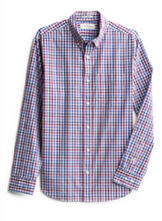
Shirt

Its Superpixel Grouping by Quickshift
While the Superpixel Grouping from Quickshift looks chaotic, it actually groups all red stripes with other red, blue with blue, etc.
Different methods of counting the number of groups
When using the k-means method, the most common question arises: how to make "k"? That is, if we need to group points into a certain number of groups, how many should we do? Several approaches have been developed to answer the question. The simplest one is the “elbow method”, but it requires manual processing of the graph, and we need an automatic solution. Gap Statistic formalizes this method, and with its help we got the best results on the “number of colors” metric, however at the expense of the accuracy of determining the base color. Since the main color is most important, we did not use it in the working program, but we plan to study this issue further.
Finally, the silhouette method is another popular k selection method. It gives results slightly worse than our algorithm, and it has one serious drawback: it needs at least 2 groups. But many clothing items only have one color.
DBSCAN
One potential solution to the question of choosing k is to use an algorithm that does not require you to choose this parameter. One popular example is DBSCAN, which looks for groups of roughly equal density in the data.

Multicolored blouse
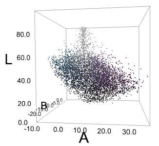
All pixels of her image are in LAB space. Pixels do not form clear cyan and violet groups.
Often we do not get such groups, or we see something like groups only because of the peculiarities of human perception. For us, the greenish-blue "cucumbers" on the blouse stand out against the purple background, but if we plot all the pixels in RGB or LAB coordinates, they won't form groups. But we tried DBSCAN anyway with different epsilon values and we got predictably poor results.
Solution from Algolia
One of the good principles of researchers is to see if anyone has already solved your problem. Leo Ercolanelli of the Algolia website published a detailed description of the solution to such a problem more than three years ago. Thanks to their generosity in the distribution of sources, we were able to try their solution ourselves. However, the results were slightly worse than ours, so we left our algorithm. They do not solve the same problem as we do: they had product images on models and against a background other than white, so it makes sense that their results differ from ours.
Color coordination
This algorithm completes the process described in our previous article. After extracting the group centers, we use Colornamer to name them and then import those colors into our internal tools. This helps us to easily visualize our products by color; we hope to incorporate this data into purchase recommendation algorithms. This process isn't perfect, it helps us get better data on our thousands of products, which in turn contributes to our primary goal of helping people find the styles they love.
Interview about the translation of the first part