Quantum theory. A universe of probability waves

Quantum theory is one of the most accurate models describing the world around us, and technical solutions developed through the use of the apparatus of quantum mechanics have firmly entered the everyday life of modern society. And it is all the more surprising that the understanding of even the basic concepts of this area of ​​knowledge comes into serious conflict with the intuition, not only of people far from science, but also of the researchers themselves, which is confirmed by a large number of different interpretations . In this article, I propose to consider the basic concepts of quantum theory from the most intuitive point of view that seemed to the author, a somewhat modified theory of probability.



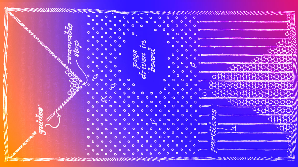
What will happen if, by analogy with the two-slit experiment, all the space on the path of the particle to the screen is filled with slits?

« — , .»



« » —

C:

1. :
2. ,

:

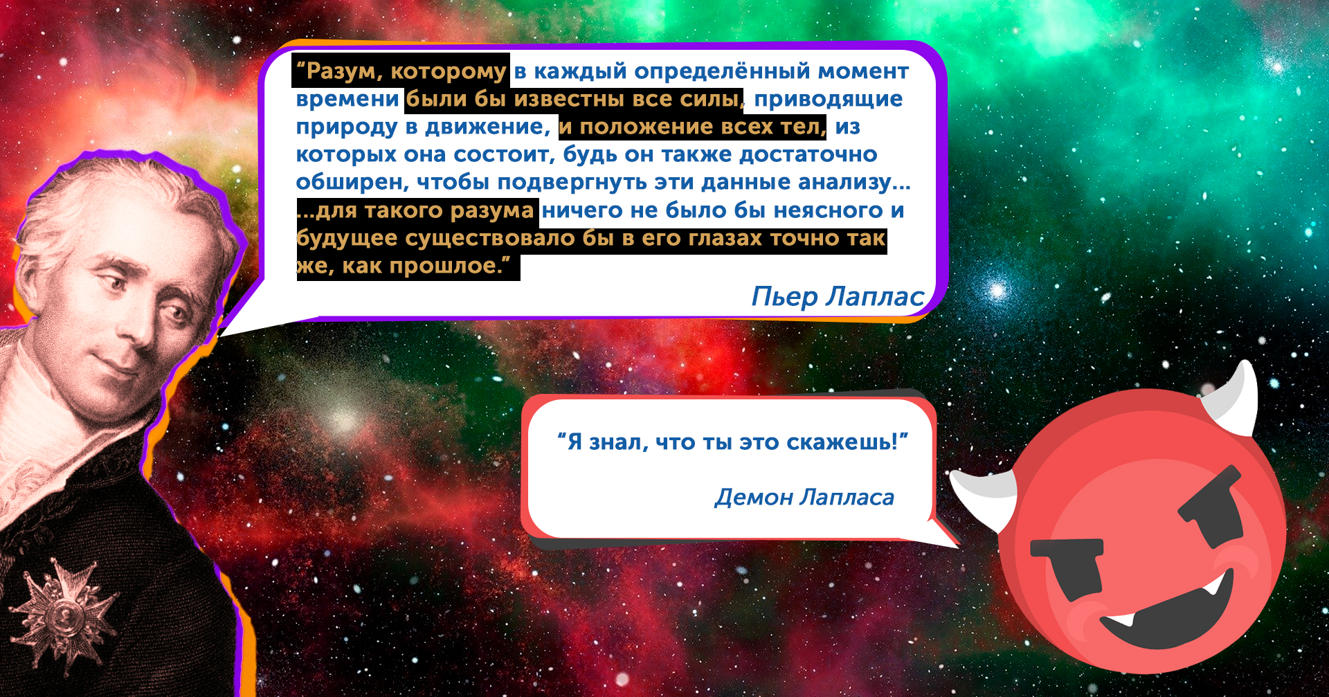
At the beginning of the 19th century, determinism dominated in the scientific picture of the world - the doctrine that the initial parameters of a system completely determine its further development. Newtonian mechanics made it possible to very accurately predict the behavior of not too large bodies moving at speeds much lower than the speed of light, and the special and general theory of relativity that appeared later made similar calculations possible for very massive objects moving at speeds close to the speeds of light.



And it was only a matter of time that the creation of Laplace's demon seemed to be a hypothetical computing device that would be able to receive the initial parameters of any system as input and calculate its standing at any moment. Scientists have already begun to anticipate an almost complete victory over uncertainty and the triumph of the human mind, although the paradoxes associated with the very possibility of the existence of Laplace's demon were already in great doubt.







But at about the same time, attempts by researchers to penetrate the structure of nature at extremely small spatial and temporal scales brought bad news for determinism. So, one of the main statements of the new quantum theory - the uncertainty principle, said that if a system has connected (commuting) parameters, then the more accurately we measure one of them, the less certainty we can determine the other.



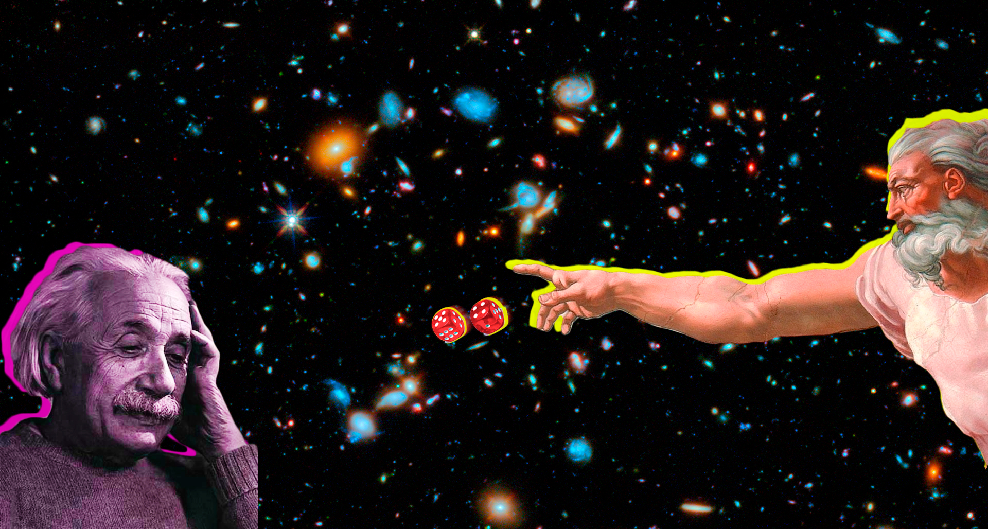
Based on these ideas, no event could be predicted with absolute accuracy, since there was some uncertainty in any measurements and this fact was not to the liking of many members of the scientific community of that time. The camp of critics was headed by Albert Einstein, who already had world authority at that time, who in correspondence with his opponent and colleague Heisenberg - Max Born, said about the possibility of the principle of uncertainty: "... In any case, I am convinced that [God] does not play dice."

Uncertainty Principle, Tattoo and Calligraphy

The operation of the uncertainty principle is often attributed to the properties of the measurement process itself, but there are more fundamental reasons and the easiest way to demonstrate them is by the example of two parameters: momentum and particle coordinates. Just as one and the same drawing can be done in two fundamentally different ways: vector and raster, that is, either in the form of lines, as, for example, in calligraphy, or in the form of a set of dots, as in the case of a tattoo. Also, the motion of a particle can be described in two alternative ways: using the momentum - the vector of mass-velocity$\$\; inline\; \$\; \backslash \; vec\; p\; =\; m\; \backslash \; vec\; v\; \$\; inline\; \$$ or using a set of space-time coordinates $\$\; inline\; \$\; \{(x\_1,\; t\_1);\; (x\_2,\; t\_2);\; ...;\; (x\_n,\; t\_n)\}\; \$\; inline\; \$$...

Left: Master of calligraphy draws the Enso symbol (円 相,), source . Right: The process of tattooing human skin, source .

And according to the principle of uncertainty, the more accurately we will fix the coordinate of an object in space-time $\$\; inline\; \$\; \Delta x\; \$\; inline\; \$$, the less information we can get about its impulse. Imagine that a ball thrown up is being photographed by several photographers, each with a different shutter speed on the camera. If the shutter speed is long, then the position of the ball in the photo will turn out to be blurry, but the vector of its movement will be clearly visible. And the shorter the shutter speed, the clearer the localization of the subject will be and, in the limit, we will get a clear ball suspended in the air and we will not be able to say at all about the trajectory along which it was moving.

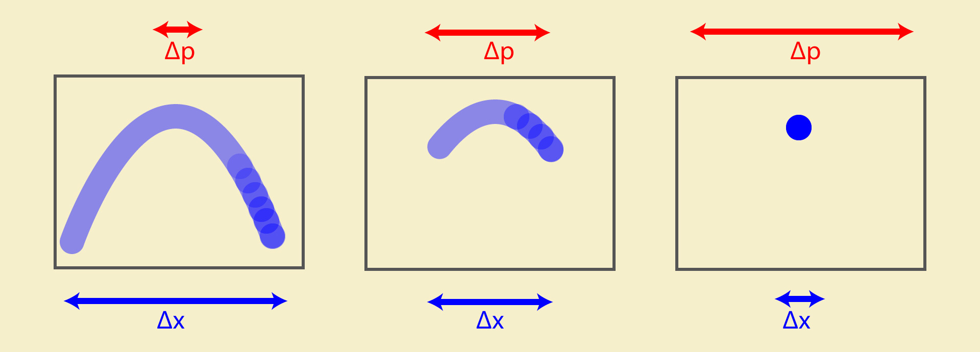
Three alternative shots of a moving object, from left to right, are shown how with an increase in the space-time interval (camera shutter speed), the amount of information about the pulse (particle trajectory) decreases.

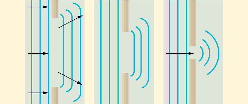
In the world of macroscopic objects, this effect is not a big problem, and if we want to set the coordinate of the car with an accuracy comparable to the size of the car itself, then there will be no problem - the car can safely enter the tunnel and at the same time maintain its predictable trajectory. But if we try to do the same, for example, with photons and start transmitting them through a decreasing slit, then at first the light spot will, as expected, become increasingly narrower, but when the size of the slit becomes comparable with the photon wavelength, then the trajectories of photons at the exit from the slit will become less and less predictable and the light spot will begin to spread out in width. In other words, the more accurately we know where the particle flew by, the less we will know about where it will move next.

Above, from left to right: interference patterns obtained with successive slit reduction, source . Bottom: diagram of the experimental setup, source .

Matter waves and their amplitudes

But it is difficult to surprise someone with the interference of a ray of light, because everyone already knows that light is a wave, and each point of the wave front will also be a source of a wave and by reducing the gap, we, according to the Huygens-Fresnel principle , get a secondary front, which, with decreasing the size of the slit will increasingly resemble a wave from a point source.

Diffraction of the forward wave front passing through the hole, source .

Indeed, any wave by its geometrical nature is not localized at one point, because to create even the simplest wave, two measurements are required - the wave amplitude (height) and the wavelength (width). And if we begin to compress the wave in height, then it will spread in length and vice versa. But more interestingly, similar experiments were carried out with particles of matter: electrons, atoms and even organic molecules, and they all also demonstrated wave diffraction.



For the first time the idea that not only photons, but in general any matter has wave properties was expressed in 1923 by the French physicist Louis de Broglie in his work " Waves and quanta". This hypothesis was partially confirmed already in 1927, as a result of the Davisson-Germer experiment, which showed the wave diffraction of electrons, which brought Louis de Broglie a well-deserved Nobel Prize in physics in 1929.



Later, the well-known two-slit experiment was delivered with electrons, which showed that the waves of matter particles can not only experience dispersion, forming secondary wave fronts, but these secondary waves can also amplify each other, meeting in the same phase or, on the contrary, mutually extinguish, meeting in antiphase, creating an interference pattern, similar to how macroscopic waves behave water waves or acoustic sound waves.

: , . : , , .

But if the waves in the water - this oscillatory motion of water particles up and down, the sound waves - is similar to the motion of the air molecules, the oscillation of which is a wave of matter, which may be a photon, atom, molecule, human? Formally, scientists did not come to a consensus on this score, nevertheless, they learned to calculate the function that describes this wave depending on the coordinate or any other parameter that can be measured and found that the square of the modulus of this function is an accurate estimate of the probability measurement results. Therefore, many scientists, including the outstanding physicist Richard Feynman, called itwave functions - with probability amplitudes. And it may seem rather strange that all matter and radiation are waves of some abstract mathematical concepts, but as we will try to show further, by accepting this statement, you can get a fairly clear explanation of many quantum effects.

Complex numbers and phase of probability

From experiments with one and two slits, we already know that in many respects the probability amplitudes behave like the most ordinary waves and can even, passing through a double slit, overlap each other, increasing or vice versa reducing the probability of a particle appearing at a point, which creates an interference pattern.

. : — . : . .

And if we define the probability of an event as the ratio of the number of outcomes leading to an event to the total number of all possible outcomes, then we get that the probability is a positive number, on the interval from zero to one, but then, if we take any two density graphs probability of finding a particle at a point, then we will see that the addition of the amplitudes of these graphs will always be greater than each of them separately and no destructive interference will be obtained.



What if we add a property to the probability waves that makes them interfere? Imagine a straight line and each point on it will correspond to the coordinate of the particle, then from each point we will perpendicularly postpone the probability corresponding to the location of the particle at this point. Connecting the point$\$\; inline\; \$\; x\; \$\; inline\; \$$and the corresponding probability we get a vector - the greater the vector length, the greater the probability of finding a particle at this point, and so that these vectors can interact, we will also add the angle of rotation to the length and take it into account when adding it.



You probably already guessed that such a construction is very similar to complex numbers, which also have a modulus - length and phase - an angle. Then each coordinate will correspond to a complex plane, in which the probability vectors will rotate like the hands of a clock, and if they look in one direction, they will add up, and if in opposite directions, they will be subtracted. By connecting the ends of these arrows, we get the shape of the wave function or the amplitude of the probability for a particle to move in a straight line in one dimension.

Animation of successive transformations that allow you to get the wave function as the sum of the probability amplitudes at points along the path of the particle (green line), first the real part of the amplitude is set, and then the phase (rotation angle) in the complex plane. Source .

Complex numbers are of the form $\$\; inline\; \$\; z\; =\; x\; +\; y\; *\; i\; \$\; inline\; \$$where the first part is $\$\; inline\; \$\; x\; \$\; inline\; \$$ called real, and the second - $\$\; inline\; \$\; y\; *\; i\; \$\; inline\; \$$- imaginary. These two components never mix, but otherwise obey the same rules as ordinary real numbers, taking into account that$\$\; inline\; \$\; i\; \$\; inline\; \$$ Is an imaginary unit and is equal to $\$\; inline\; \$\; \backslash \; sqrt\; \{-1\}\; \$\; inline\; \$$...



One of the basic axioms of quantum theory, called Born's rule , states that the square of the modulus of the wave function gives us a probability density function , that is, in our example, the probability distribution of finding a particle depending on the coordinate.



A quick refresh in memory, the modulus of a complex number is the distance from the origin -$\$\; inline\; \$\; (0,\; 0i)\; \$\; inline\; \$$ to the point with coordinates $\$\; inline\; \$\; (x;\; yi)\; \$\; inline\; \$$, i.e: $\$\; inline\; \$\; \backslash \; sqrt\; \{x\; ^\; 2\; +\; (y\; \backslash \; sqrt\; \{-1\})\; ^\; 2\}\; \$\; inline\; \$$, it's clear that $\$\; inline\; \$\; (\backslash \; sqrt\; \{-1\})\; ^\; 2\; =\; -1\; \$\; inline\; \$$, but we will not write off the imaginary unit for now, but find the square of the modulus:

$\$\; inline\; \$\; \backslash \; left\; (\backslash \; sqrt\; \{x\; ^\; 2\; +\; (y\; \backslash \; sqrt\; \{-1\})\; ^\; 2\}\; \backslash \; right)\; ^\; 2\; =\; x\; ^\; 2\; +\; (y\; \backslash \; sqrt\; \{-1\})\; ^\; 2\; =\; (x\; +\; y\; \backslash \; sqrt\; \{-1\})\; (xy\; \backslash \; sqrt\; \{-1\})\; \$\; inline\; \$$

We get that the square of the modulus of a complex number is its product by the same complex number, which differs only in the sign before the coefficient of the imaginary part $\$\; inline\; \$\; z\; =\; xy\; *\; i\; \$\; inline\; \$$... Such pairs of numbers are called complex conjugate and are mirror reflections of each other, corresponding to the rotation of vectors in the complex plane by equal angles, but in opposite directions.

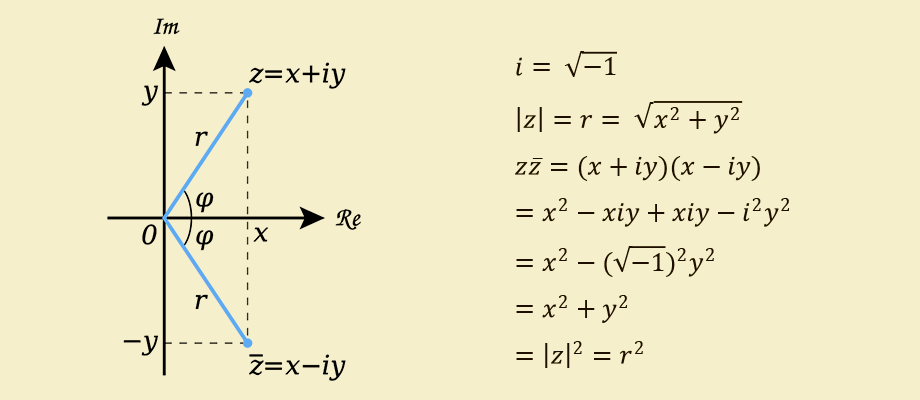
Where: $\$\; inline\; \$\; \backslash \; overline\; z\; \$\; inline\; \$$ - complex conjugate number

The real world of imaginary units

Here's what we already understood: the wave function assigns a certain complex number to each coordinate. Actually, this is what the wave functions do - they put in correspondence to some measurable parameter a complex number, the angle of rotation of which is called the phase. The phases of complex numbers are responsible for the interference effects of amplification and attenuation of probabilities, which are obtained by multiplying the wave function by its mirror reflection - complex conjugation.



When asked why the square of the modulus of the wave function gives the probability density, quantum theory usually answers - shut up and countbecause the square of the modulus makes a real out of a complex number. Of course, this answer does not suit us at all, because from a complex number you can get a real one by simply taking its modulus, so I would like to understand the meaning of squaring the modulus.



Let's imagine that we know nothing about either the wave function or the probability density function, but simply made a lot of observations and marked with dots where and with what frequency the particle appears. At the same time, we understand that the resulting distribution should be described by some kind of graph of the probability density function and it would be extremely useful to know this function itself.



To find out which function corresponds to our points, let's go the simplest way and begin to fit the answer to the data, that is, to select polynomials that will pass through the maximum number of available points. Let's start with two points and select for them the coefficients of the polynomial of the first degree, that is, the linear function$\$\; inline\; \$\; y\; =\; ax\; +\; b\; \$\; inline\; \$$because the line will pass exactly through our two points. If there are points that do not lie on this line, then we take a second order polynomial$\$\; inline\; \$\; y\; =\; ax\; ^\; 2\; +\; bx\; +\; c\; \$\; inline\; \$$the graph of which are various parabolas, choosing the coefficients we are guaranteed to get at least three points, one of which will be a vertex, and the other two will lie on the sides. Then we again check whether there are still points lying outside the graph, if so, we repeat by increasing the degree of the polynomial by one more and so on, the logic is clear, the polynomial of degree$\$\; inline\; \$\; n\; \$\; inline\; \$$ guaranteed to pass through $\$\; inline\; \$\; n\; +\; 1\; \$\; inline\; \$$points and as a result we can choose a polynomial that will cover all our points. There is even a special theorem - Weierstrass ' approximation theorem , which confirms that this is possible.

An example of fitting points taken from the probability density function of a normal distribution with polynomials of various degrees, from linear to 18th degree, using the numpy.polyfit function . You can make sure that the degree of the polynomial corresponds to the number of points through which its graph passes.

Python code:

from numpy import *
from matplotlib.pyplot import *
from mpl_toolkits.axes_grid.axislines import SubplotZero


mu, sigma = 0, 0.1
x = np.arange(-1,1,0.02)
y = 1/(sigma * np.sqrt(2 * np.pi))*np.exp( - (x - mu)**2 / (2 * sigma**2) )

y1 = poly1d(polyfit(x,y,1))	# linear
y2 = poly1d(polyfit(x,y,2))	# quadratic
y3 = poly1d(polyfit(x,y,3))	# cubic
y4 = poly1d(polyfit(x,y,4))	# 4th degree
y5 = poly1d(polyfit(x,y,10))	# 10th degree
y6 = poly1d(polyfit(x,y,18))	# 18th degree

fig = figure(figsize=(20,8), facecolor='#f4efcb', edgecolor='#f4efcb')
ax = SubplotZero(fig,111)
fig.add_subplot(ax)

ax.plot(x,y1(x),'r',label=u'')
ax.plot(x,y2(x),'g',label=u'')
ax.plot(x,y3(x),'orange',label=u'')
ax.plot(x,y4(x),'b',label=u'$4$ ')
ax.plot(x,y5(x),'c',label=u'$10$ ')
ax.plot(x,y6(x),'m',label=u'$18$ ')
ax.plot(x,y,'k.',label=u'')

ax.set_xlabel(u'x')
ax.set_ylabel(u'y')
ax.set_facecolor('#f4efcb')
ax.minorticks_on()
ax.legend(frameon=False,loc=8,labelspacing=.2)
ax.annotate('  18 :'+'\n'+str(y6.coeffs), xy = (-1,1.2))

setp(ax.get_legend().get_texts(), fontsize='large')

fig.savefig("Curve fitting.svg",bbox_inches="tight",pad_inches=.15)

And since the probability density can be approximated by a polynomial, then surely this polynomial also has roots, and another wonderful theorem, the main theorem of algebra says that yes, any polynomial must have solutions in complex numbers, and if the roots are real, then this simply means that the imaginary part is equal to zero (the vectors will have a zero rotation angle), since the set of real numbers is completely contained in the set of complex$\$\; inline\; \$\; \backslash \; mathbb\; \{R\}\; \backslash \; subset\; \backslash \; mathbb\; \{C\}\; \$\; inline\; \$$...



And if any complex number$\$\; inline\; \$\; z\; =\; x\; +\; y\; *\; i\; \$\; inline\; \$$ is a root of some polynomial, then automatically the root of the same equation is the number conjugate to it $\$\; inline\; \$\; \backslash \; overline\; z\; =\; xy\; *\; i\; \$\; inline\; \$$, another theorem tells us about this - the theorem on complex conjugate roots .



For example, let's imagine that the probability density is described by a polynomial of the second degree$\$\; inline\; \$\; x\; ^\; 2\; +\; 5\; *\; x\; +\; 6.5\; \$\; inline\; \$$and find its roots. By the formula for the roots of a quadratic equation$\$\; inline\; \$\; x\_\; \{1,2\}\; =\; \backslash \; frac\; \{-b\; \backslash \; pm\; \backslash \; sqrt\; \{b\; ^\; 2-4ac\}\}\; \{2a\}\; \$\; inline\; \$$by substituting the coefficients $\$\; inline\; \$\; a\; =\; 1,\; b\; =\; 5,\; c\; =\; 6.5\; \$\; inline\; \$$ and we obtain in the form of a solution two conjugate complex numbers $\$\; inline\; \$\; x\_1\; =\; -5\; /\; 2\; +\; i\; /\; 2\; \$\; inline\; \$$, $\$\; inline\; \$\; x\_2\; =\; -5\; /\; 2\; -\; i\; /\; 2\; \$\; inline\; \$$, as the theorem on conjugate roots asserted to us.



On the other hand, knowing the roots and using Vieta's formulas, we can decompose the same square trinomial as follows:$\$\; inline\; \$\; x\; ^\; 2\; +\; bx\; +\; c\; =\; (x-x\_1)\; (x-x\_2)\; \$\; inline\; \$$it is easy to check that this is true, substituting the obtained values ​​and opening the brackets, we get the original polynomial. But at the same time, on the right side of the Vieta formula, we got the product of two conjugate complex numbers, which is the square of the modulus. In principle, the same logic can be extended to other degrees of polynomials, the main thing is that the roots will always go in pairs, and their multiplication will be used to obtain the original polynomial.



Of course, this is a very loose reasoning, designed to somehow comprehend what is happening and, using a simple example, show that complex numbers are fully justified, and their conjugate products can give something similar to a probability density.

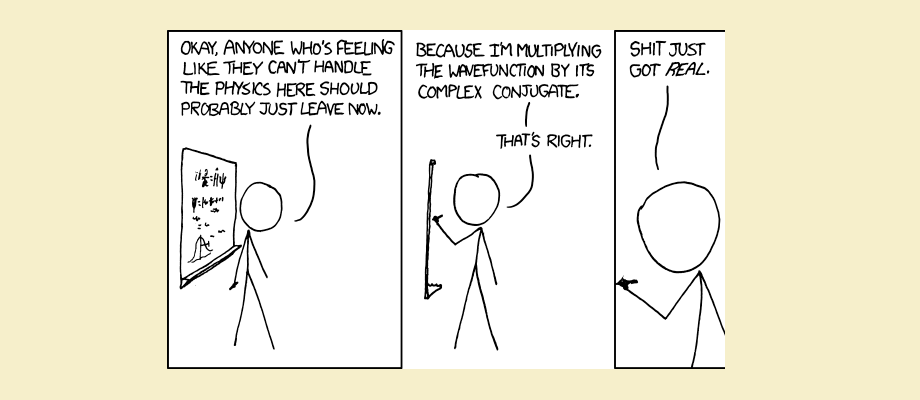
A comic strip with a joke on the topic of real numbers and the multiplication of a wave function by its own complex conjugation. A source

Okay, let's assume we have some idea of ​​how the probability amplitudes work, why they are complex, and how ordinary probabilities are derived from them. And we can move on to the question of what these probabilities predict for us, that is, about the results of measurements .

Wave function and probability density

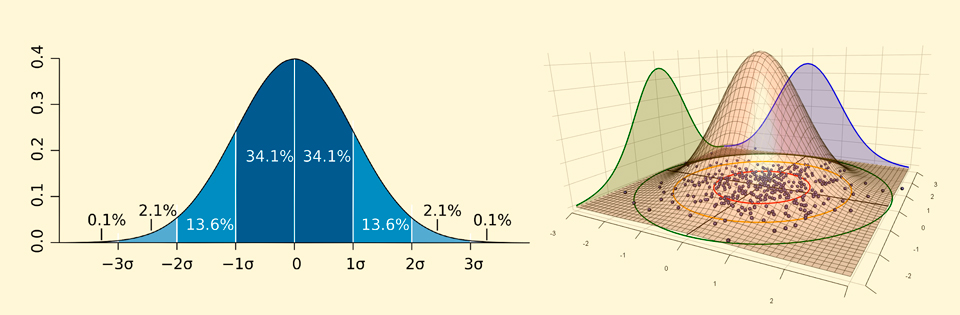
By obtaining the probability density of finding a particle in a certain coordinate, we predict the frequency with which we will observe the particle at different points. For example, if the probability density is described by a Gaussian curve, as on the left side of the figure below, then in$\$\; inline\; \$\; 68\; \backslash \%\; \$\; inline\; \$$ cases we will see that the particle appears on the interval from $\$\; inline\; \$\; -1\; \backslash \; sigma\; \$\; inline\; \$$ before $\$\; inline\; \$\; +\; 1\; \backslash \; sigma\; \$\; inline\; \$$and in $\$\; inline\; \$\; 95\; \backslash \%\; \$\; inline\; \$$ cases on the segment from $\$\; inline\; \$\; -2\; \backslash \; sigma\; \$\; inline\; \$$ before $\$\; inline\; \$\; +\; 2\; \backslash \; sigma\; \$\; inline\; \$$etc. Which, in the case of a two-dimensional symmetric distribution, shown on the right, will give a higher detection density of a particle in some circular area in the center and a low density as it moves away from the center:







A fairly straightforward scheme: the wave function of the coordinate sets the shape of the distribution, which then tells us the probabilities of measuring a particle at a point in space. Nevertheless, such an interpretation can lead to strange contradictions and it is sometimes more natural to think of particles as waves of probability amplitudes. For example, the picture below, on the left, shows what the probability density looks like for an electron interacting with a hydrogen nucleus. In accordance with this graph, you can get the shape of the so-called electron orbitals - areas around the nucleus of an atom in which interaction with an electron is most likely, shown on the right:





Left: probability density curves of finding an electron around a single proton, for three energy levels$\$\; inline\; \$\; 1s,\; 2s,\; 3s\; \$\; inline\; \$$... Right: shows an example of what the distributions of points would look like when measuring the coordinate of an electron. Source .



In the figure above, you can see how the shapes of the orbitals change depending on the energy level of the electron - the higher the energy of the electron, the, first, the larger the radius of the shell, which is quite understandable, because the more energy, the stronger the electron can resist the attraction of the nucleus and the further from the nucleus, it can interact, but at the same time, to each new energy level, a section with zero probability is added, called a node, so, for example, the orbital of an electron at the 3rd energy level has the form of a layered sphere containing two zones inside, the probability detection of an electron in which is zero.





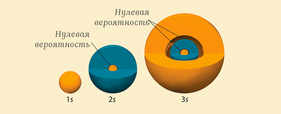
The contour of the probability of finding an electron in the vicinity of the nucleus of a hydrogen atom for three energy levels from left to right: 1s, 2, s 3s. Source .



Such a probability distribution looks very strange, because it is impossible to get from one sphere to another without crossing the nested one between them.



But if you think of an electron as an amplitude of probability, then everything is explained quite naturally, in the picture below the wave function of the radius of an electron around the hydrogen nucleus, calculated in one dimension, for three energy levels.







Looking at the graphs of the wave function, it is easier to understand that an electron held by the nucleus of an atom is a standing wave and, like any standing wave, it will have so-called nodes (node ) - zones where the amplitude will be zero as a result of interference with the reflected wave.



An example of the formation of interference nodes (red dots) in a one-dimensional standing wave, source .



And if a one-dimensional wave, as in the animation above, still does not resemble the shape of a layered three-dimensional electron shell of a hydrogen atom, then I propose to imagine a wave on a two-dimensional plane propagating from a point source. So, to see the full shape of such a two-dimensional wave, you need to look at it in threemeasurements. And for an inhabitant of a two-dimensional world, such a wave will be just a set of circles diverging from the center. Similarly, with three-dimensional waves - they live in four dimensions, but for us they will look like diverging three-dimensional spheres.





Right: Animation of a wave propagating over a 2D surface. Left: An example of what the projection of this wave onto a plane would look like.

Quantum decoherence barrier

Abraham Pais is an eminent physicist and historian of science who collaborated with a galaxy of 20th century science legends, including: John von Neumann, Albert Einstein, Niels Bohr, Max Born, Paul Dirac, Wolfgang Pauli and many others. describing one of the dialogues concerning the problem of the observer in quantum physics, he quoted a question posed to him by Einstein:

"Do you really think the moon only exists when you look at it?" (Rev. Mod. Phys. 51, 863-914 (1979), p. 907).

And indeed the ancient philosophical dilemma about the existence of objective reality, with the discovery of the quantum properties of our world, has become even more urgent. The wave function makes it possible to predict the measurement result with the required accuracy, but does it exist in isolation from the context of the measurement and the observer, and how can this be verified?



First of all, it is necessary to define what observation and measurement are . To measure the size of an object, we apply a ruler to it, to measure the temperature - we apply a thermometer to measure the speed - we send an electromagnetic wave towards it.



In all these cases, we need the interaction of the measured object with some other object, the state of which we can preliminary prepare, such an object will be called a measuring system. They shook off the thermometer - prepared the measuring system, put the armpit - made an interaction, and then evaluated how much the state of the control system had changed. This is a general principle, any measurement is the interaction of the measured system with the control one.



Any observation is also a measurement, observing something we get information about the object using the measuring systems built into our body, which also interact with the object. If we look at an object, then we interact with photons emitted by this object, which, falling on the retina of the eye, lead to a complex cascade of interactions and the launch of a nerve signal entering the brain.

« ? … . , , , . , … : “ , , ”».



«. » —

The principle of superposition of waves tells us that when two or more waves meet at one point in space, the result of the interaction will be a new wave, which is the sum of their amplitudes. Then, the measurement result will always be some superposition of the wave functions of the measured and the measuring system.



Now a reasonable question arises: if we accept the assertion that everything consists of waves of probability amplitudes, then why do we live so boringly not observe wave properties such as superposition and interference in macroscopic objects that surround us?



To answer this question, let us look again at the double-slit experiment: electrons fly through the double slit one at a time and hit the screen, are marked on it with a dot; when this process is repeated many times, the dots form an interference pattern that corresponds to the passage of a wave through two slits.

Left: animation of the interference pattern from the passage of a wave through a double slit, source . Right: Results of an experiment on recording single electrons after passing through a double slit. Source: New Journal of Physics, Volume 15, March 2013 .

But if we want to know which of the slits the electron passes through and put a measuring device in front of one of them, then the interference pattern on the screen will disappear, and we will see only two peaks on the screen. All this is puzzling, and one might get the impression that there is some special rule that tells the electron that if no one is looking, then it propagates in the form of a wave, and when they try to measure it, it turns into a localized particle. It sounds very strange, because keeping so many complex rules for one simple electron is not at all in the spirit of nature.

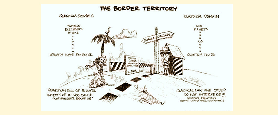
A cartoon that pokes fun at the separation of phenomena into quantum and classical. Source (http://www.bourbaphy.fr/zurek.pdf)

What if we only apply the principle of superposition, can we get the same observed effects? So if first we have a wave function that describes the coordinate of the interaction of a single electron with the screen$\$\; inline\; \$\; |\; \backslash \; psi\; \backslash \; rangle\; \$\; inline\; \$$, then after passing through the double slit, it will be the sum of two wave functions - passed through the slit $\$\; inline\; \$\; 1\; \$\; inline\; \$$ and through the gap $\$\; inline\; \$\; 2\; \$\; inline\; \$$, then the general state can be written as a superposition of these two states$\$\; inline\; \$\; \backslash \; psi\; =\; \backslash \; psi\_1\; +\; \backslash \; psi\_2\; \$\; inline\; \$$...



In the case of one wave function, in order to find the probability of the particle interaction at a point, we multiply the value of the wave function at this point by its own complex conjugation, the imaginary units cancel out, and we get the classical probability:

$$$p(x_j)=|\psi(x_j)|^2= z _j^* z_j= |z_j|^2$

In the case of a superposition of two possible routes, we multiply the sum of the wave functions:

$$$p(x_j)=|\psi_1(x_j)+\psi_2(x_j)|^2=$

$$$= (z1 _j^*+ z2 _j^*)(z1 _j+ z2 _j)=$

$$$= |z1 _j|^2+z1 _j^*z2 _j+z2 _j^*z1 _j+|z2 _j|^2$

In the expression above, in addition to the modules of complex numbers, we also received terms of the form: $$$z1 _j^*z2 _j$ and $$$z2 _j^*z1 _j$ products of different complex numbers, the result of which will depend on the phase angle $$$φ$ these complex numbers:

$$$z1z2=|z1|⋅|z2|[cos(φ1+φ2)+isin(φ1+φ2)]$

To understand how the phases of the two alternative routes will interact, imagine the phase as an arrow that rotates at a given speed, as the wave propagates, one full turn of the arrow corresponds to the wavelength, and the rotation speed corresponds to the frequency.

The black arrow shows a comparison of the "rotation rate" of the phases of two wave packets with different source frequencies .

Since two alternative wave functions are obtained by dividing one original, it is reasonable to assume that their frequency and wavelength will be the same and the arrows of the resulting waves will rotate at the same speed. Based on this, the phase difference, when meeting at a point on the screen, will depend only on the difference in the distance traveled by the wave to this point.



This means that at a point located at an equal distance from each of the holes, the waves will meet with the same position of the arrows, that is, in one phase and in this place we will see a peak in the interference pattern, and at the point where the difference in the distances traveled will be half the length waves - the arrows of the waves will meet in opposite positions and destructive interference will occur, which will give a dark spot. If you move a little more to a point where the difference is an entire wavelength, the arrows will coincide again, and so on.

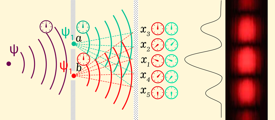
The appearance of two alternative possibilities of hitting the screen leads to the division of the original wave function into two with the same phases, shown in the form of a dial with an arrow. The same phase implies the same rotation speed of the arrow. When hitting a point on the screen at the moment of the same position of the arrows, the waves interfere constructively, if the arrows are directed in opposite directions, destructive interference occurs.

Where does the interference disappear when we measure, which gap does the electron pass through? After passing through the detector, not two, but many more different alternative variants of the wave function appear, because even if the detector is microscopic, it will still consist of a huge number of atoms, for example, even one hundredth of a gram of iron contains about$$$10^{20}$atoms, but the specific number is not important to us now, the main thing is that a huge variety of different interaction options appear, which depend on the specific state of the detector particles, and each alternative state will give its own alternative version of the wave function.



Also take$$$p(x_j)=|\psi(x_j)|^2$ Is the probability of an electron hitting the coordinate $$$x_j$ on the screen, after passing through the detector and again write this probability through the superposition of all possible alternative trajectories:



$$$\psi(x) = \psi_1(x)+\psi_2(x)+...+\psi_n(x)$where $$$n$ - a very large number of different options for the state of the detector.

$$$p(x_j)=|\psi_1(x_j)+\psi_2(x_j)+...+\psi_n(x_j)|^2=$

$$$= (z1 _j^*+ z2 _j^*+...zn _j^*)(z1 _j+ z2 _j+...+zn _j)=$

$$$= (\sum_{j=1}^n z_j^*)(\sum_{j=1}^n z_j)$

For clarity, we write the result of multiplying these sums in the form of a matrix from $$$n^2$ elements:

$$$\begin{bmatrix} (z1^*)(z1) & (z1^*)(z2) & \cdots & (z1^*)(zn) \\ z2^*)(z1) & (z2^*)(z2) & \cdots & (z2^*)(zn) \\ \vdots & \vdots & \ddots & \vdots \\ (zn^*)(z1) & (zn^*)(z2) & \cdots & (zn^*)(zn) \end{bmatrix}$

Total we got $$$n$ - classical probabilities along the diagonal and $$$(n^2-n)$and interference terms, and all this together gives the probability of an electron hitting for one point. But in this case the interference terms will no longer have the same phase, as in the previous case, when the wave either passed through the slit without interaction, or was completely reflected. Now, passing through a detector consisting of various particles not synchronized with each other, the resulting wave functions will also have random - incoherent phases.



Such desynchronized states are called mixed states.). And although the wave functions of mixed states will also interfere, the result of the interference will no longer depend on the distance traveled by the wave, and at each point of the screen one can expect the same and very large number of both constructively and destructively interfering terms, which on average will give their zero contribution ... Just as the impacts of gas molecules do not move the object from its place, since at each moment of time the object receives approximately the same number of impacts from all directions.

Loss of coherence of the wave function $\$\; inline\; \$\; 1\; \$\; inline\; \$$ after passing the detector $\$\; inline\; \$\; d\; \$\; inline\; \$$ leads to zeroing of the contribution of interference terms at points on the screen and the appearance of a pattern corresponding to the superposition of two Gaussian peaks.

In the general case, any interaction of a quantum system with the external environment inevitably and very quickly leads to mixing of states, and, as a result, to phase desynchronization and averaging of alternative states - decoherence.



Therefore, our version of the answer to the question: why do we not observe quantum effects in macroscopic objects under normal conditions? To obtain a superposition of the states of a macroscopic object, it is necessary to completely isolate it from interaction with the external environment, including placing it in a complete vacuum, cooling to ultra-low temperatures and shielding from different fields, which is very difficult to implement in practice. In other words, Schrödinger's cat would have died even while preparing the conditions necessary for creating its superposition, long before the radioactive particle would decay, breaking the ampoule with poison.

A bit of quantum cryptography

The fact that your smartphone still does not have a quantum processor, you also have to blame decoherence. After all, even the most modern quantum computers take up an entire room, and the bulk of their designs are cryogenic cooling and shielding systems.

D-Wave 2000Q quantum computer construction diagram, source .

But if decoherence is a big problem in creating quantum computers, then in cryptography the inevitable change in the wave function during measurement came in handy. For example, if we take a photon as a quantum bit, then, depending on the angle of its polarization, we can choose two different coding options for zero and one:

• $$$0$ - vertical polarization, $$$1$ - horizontal;
• $$$0$ - diagonal polarization, $$$1$ - antidiagonal.

Let's designate these two coding methods as two bases: $$$VH$ and $$$DA$, respectively. Then if the sender - Alice encodes a bit in the basis$$$VH$, that is, it sends either a horizontally polarized photon or a vertical one, then the receiver Bob will need to pass the received photon through a linear polarizing filter, which completely blocks vertical polarization.



Then if a photon flies through the polarizer and hits the detector, then we know for sure that it was horizontally polarized$$$0$, and if it does not fly by - vertical - $$$1$... Similarly, if you turn the polarizing filter to a vertical position, then it will block$$$100\%$ horizontally polarized photons.

Left: A vertically oriented photon is blocked by a linear polarizing filter. Right: When you turn the polarizing filter to$$$90°$a vertically polarized photon passes freely. Source .

So far, everything is fully consistent with the classic picture coding system. But due to the principle of superposition, we can represent a diagonal photon as a composition of horizontal and vertical polarization, and if we then pass it through a polarizer oriented to filtering vertical photons, then the output will only have a horizontal component with an amplitude$$$1/2$ from the original, which in the case of a single photon will correspond to $$$50\%$ the probability of passing through the filter.

On the left: a diagonal photon (red arrow) presented as a composition of the horizontal and vertical components (pink and purple arrows) of the electromagnetic field. Right side: A linear polarizing filter blocks the vertical component of a diagonal photon and outputs a horizontally polarized photon. A source

This means that if we encode each next bit in a randomly selected basis, then the receiver will also need to change the rotation of the polarizing filter, because if he measures a photon encoded in a horizontal - vertical basis $$$VH$ with the filter turned under $$$45°$then it will receive $$$0$ and $$$1$ randomly with probability $$$50\%$, which is analogous to a complete loss of information.

Passing through a vertical linear polarizer, the diagonal and antidiagonal photons lose the horizontal component and the output is a horizontal photon with the amplitude $\$\; inline\; \$\; 1/2\; \$\; inline\; \$$from the original. Source .

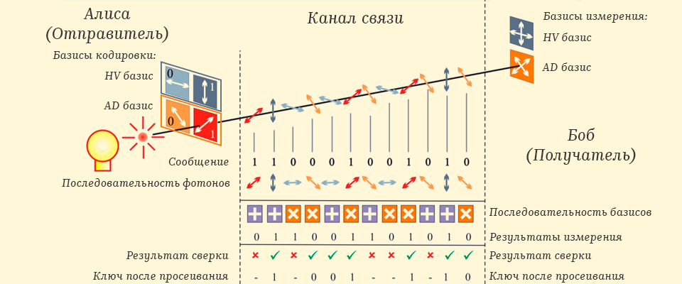
The first quantum cryptography protocol is based on this principle - $\$\; inline\; \$\; BB84\; \$\; inline\; \$$that allows you to transfer the encryption key over an open channel. So if Alice needs to send Bob a message consisting of n characters, then the most reliable way would be to translate each of the characters into a binary code, and then take a sequence of random zeros and ones of the same length and perform a bitwise addition XOR, that is, if the characters with the same indices coincide then as a result we get 0, and if they differ then$\$\; inline\; \$\; 1\; \$\; inline\; \$$...



So, Alice receives an encrypted message and a key, if the recipient Bob also has a key, then he can do the XOR operation again and get the original message. Quantum cryptography physics just allows you to exchange a key, so in the algorithm$$$BB84$not one but two sequences of random bits are generated at once with some margin regarding the message. The first sequence indicates in which basis the photon, which is the quantum bit of the key sent by Alice-Bob, will be encoded . Then Bob , receiving photons, also using a random sequence, chooses in which basis to measure each photon, while he will receive an incorrect result with the probability$$$25\%$...



After completing the transfer of the quantum key, it is necessary to get rid of errors, for this, the so-called key sifting procedure is applied , when Alice sends Bob a sequence of bases in which the key was encoded simply through the classical channel, after which Bob verifies this sequence with the one in which he measured the photons upon receiving the key and sends back to Alice those positions that turned out to be erroneous. Alice crosses out the erroneous positions and the obtained key is used further for encryption.



The quantum trick is that if an eavesdropper is connected to the channel, say - Eve, which will intercept a photon, measure it and direct it further to Bob , then measuring the intercepted photons with an incorrectly chosen basis, it will also inevitably destroy the superposition. Thus, even after sifting, there will still be errors in Bob's key that can be detected during the verification process, when Alice sends a fragment of her key to Bob via the classical channel, if no errors are found as a result of verification, then it will be possible to use the key with confidence for messaging.

Logic diagram of the encryption algorithm $$$BB84$... Source .

Conclusion

I hope that from this article you were able to glean some information and get a general impression of how quantum theory from an extravagant idea became one of the most complete and accurate physical models of our Universe. And finally, for those wishing to dive deeper into the topic, I would like to recommend several resources and books:

• "Physics and Philosophy" - Werner Heisenberg, comprehension of quantum theory, as seen by one of its most prominent founders.
• QED - A Strange Theory of Light and Matter is a classic book by the brilliant Richard Feynman, which is based on popular science lectures given by him in the 60s at the California Institute of Technology (Caltech).
• « » — , , , — .
• « » — - , , .
• Physics Videos by Eugene Khutoryansky — YouTube , , , .
• Minute phisics — , , , : , , .
• 3Blue1Brown - Channel of Oxford alumnus Grant Sanderson, a great combination of easy-to-understand presentation and unique visualization of concepts from: quantum physics , linear algebra , neural networks . Grant is also the author of a course on multivariate calculus available on the site of the non-profit project Khan Academy .