In a good city near Moscow, there is a bad railway crossing. During rush hour not only it rises, but also neighboring intersections and roads. Driving once again, I wondered - what is its capacity and can something be changed?

For the answer, we will delve a little into the regulations and theory of traffic flows, analyze GPS and accelerometer data using Python and compare theoretical calculations with experimental data.
Content
- 1 Initial data
- 2 Theory of traffic flow
- 3 Data collection and analysis
- 3.1
- 3.2
- 3.2.1
- 3.2.2
- 3.3
- 4
1.
, 10 /. .
Jupyter Notebook GitHub'.

:
import pandas as pd
import numpy as np
import glob

#!pip install utm
import utm

from sklearn.decomposition import PCA
from scipy import interpolate

import matplotlib.pyplot as plt
import seaborn as sns
sns.set(rc={'figure.figsize':(12, 8)})
import plotly.express as px

#  Mapbox    Plotly
mapbox_token = open('mapbox_token', 'r').read()
2.
.
— 1 .
— .
— , .
— , - .
:
.
« » . , 2005 . , .

218.2.020-2012 " ".
, :
— , , , .
, :
, , .
2 :
- ;
- .
:
- :
,
,
– () , – , – , , — . ( ): .
- :
,
— ( ), — () ( ). 218.2.020-2012 —
#
diagram1 = pd.read_csv('  .csv', sep=';', header=None, names=['P', 'V'], decimal=',')
diagram1_func = interpolate.interp1d(diagram1['P'], diagram1['V'], kind='cubic')
diagram1_xnew = np.arange(diagram1['P'].min(), diagram1['P'].max())

#
diagram2 = pd.read_csv(' .csv', sep=';', header=None, names=['P', 'Q'], decimal=',')
diagram2_func = interpolate.interp1d(diagram2['P'], diagram2['Q'], kind='cubic')
diagram2_xnew = np.arange(diagram2['P'].min(), diagram2['P'].max())
def density_Tanaka(V):
#
V = V * 1000 / 60 / 60 # / /
L = 5.7 #
c1 = 0.504 #
c2 = 0.0285 #**2/
return 1000 / (L + c1 * V + c2 * V**2) # ./
def density_Grindshilds(V):
#
pmax = 85 # ./
vmax = 60 # /
return pmax * (1 - V / vmax) # ./#
V = np.arange(1, 80) # /
V1 = np.arange(1, 61) # /
fig, (ax1, ax2) = plt.subplots(1, 2, figsize=(16, 8))
ax1.plot(density_Tanaka(V), V, label=" ")
ax1.plot(density_Grindshilds(V1), V1, label=" ")
ax1.plot(diagram1_xnew, diagram1_func(diagram1_xnew), label=". ")
ax1.set_xlabel(r' $\rho$, /')
ax1.set_ylabel(r' $V$, /')
ax1.legend()
ax2.plot(density_Tanaka(V), density_Tanaka(V) * V, label=" ")
ax2.plot(density_Grindshilds(V1), density_Grindshilds(V1) * V1, label=" ")
ax2.plot(diagram2_xnew, diagram2_func(diagram2_xnew), label=". ")
ax2.set_xlabel(r' $\rho$, /')
ax2.set_ylabel(r' $Q$, /')
ax2.legend()
plt.show()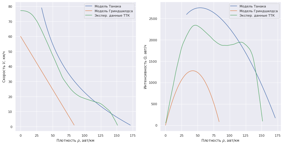
. .
3.
3.1
, . Enter, :
%%writefile "key-logger.py"
import pandas as pd
import time
import datetime

class _GetchUnix:
    # from https://code.activestate.com/recipes/134892/
    def __init__(self):
        import tty, sys

    def __call__(self):
        import sys, tty, termios
        fd = sys.stdin.fileno()
        old_settings = termios.tcgetattr(fd)
        try:
            tty.setraw(sys.stdin.fileno())
            ch = sys.stdin.read(1)
        finally:
            termios.tcsetattr(fd, termios.TCSADRAIN, old_settings)
        return ch

def logging():
    path = 'logs/keylog/'
    filename = f"{time.strftime('%Y-%m-%d %H-%M-%S')}.csv"
    path_to_file = path + filename
    db = []
    getch = _GetchUnix()
    print('...')
    while True:
        key = getch()
        if key == 'c':
            break
        else:
            db.append((datetime.datetime.now(), key))
    df = pd.DataFrame(db, columns=['time', 'click'])
    print(df)
    df.to_csv(path_to_file, index=False)
    print(f"\nSaved to {filename}")

if __name__ == "__main__":
    logging()
20 . 2 , . . 100%:
files = glob.glob('logs/keylog/*.csv')
keylogger_data = []
print(f'  - {len(files)} .')
for filename in files:
    df = pd.read_csv(filename, parse_dates=['time'])
    keylogger_data.append(df)
keylogger_data = pd.concat(keylogger_data, ignore_index=True)
keylogger_data.head()| time | click | |
|---|---|---|
| 0 | 2020-09-29 16:24:02.691189 | d |
| 1 | 2020-09-29 16:24:05.186670 | a |
| 2 | 2020-09-29 16:24:07.157702 | d |
| 3 | 2020-09-29 16:24:11.506961 | a |
| 4 | 2020-09-29 16:24:14.206266 | a |
"a" — , 'd' — .
:
keylogger_data['time'] = keylogger_data['time'].astype('datetime64[m]')
keylogger_per_min = keylogger_data.groupby(['click', 'time'], as_index=False).size().reset_index().rename(columns={0:'size'})
keylogger_per_min.head()| index | click | time | size | |
|---|---|---|---|---|
| 0 | 0 | a | 2020-09-29 16:24:00 | 12 |
| 1 | 1 | a | 2020-09-29 16:25:00 | 13 |
| 2 | 2 | a | 2020-09-29 16:26:00 | 9 |
| 3 | 3 | a | 2020-09-29 16:27:00 | 18 |
| 4 | 4 | a | 2020-09-29 16:28:00 | 14 |
sns.catplot(x='click', y='size', kind="box", data=keylogger_per_min);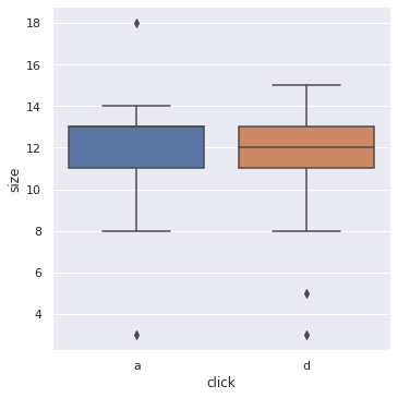
print(f"  : {keylogger_per_min['size'].mean():.1f} ./ \
 {keylogger_per_min['size'].mean() * 60:.1f} ./")
: 11.7 ./ 700.0 ./
.
— 700 ./ 10 / ( 50 / ) — .
plt.plot(V1, density_Grindshilds(V1)*V1, label=" ")
plt.xlabel(r' $V$, /')
plt.ylabel(r' $Q$, /')
plt.show()
3.2
Android GPSLogger csv . ( ) GPS — Physics Toolbox Suite.
50 . — .
, — .
GPSLogger
GPSLogger , :
- time — ;
- lat lon — , ;
- speed — , ;
- direction — , .
files = glob.glob('logs/gps/*.csv')
gpslogger_data = []
print(f'    GPS - {len(files)} .')
for filename in files:
    df = pd.read_csv(filename, parse_dates=['time'], index_col='time')
    if df.iloc[10, 1] < df.iloc[-1, 1]:
        df['direction'] = 0 #
    else:
        df['direction'] = 1 #
    gpslogger_data.append(df)
gpslogger_data = pd.concat(gpslogger_data)
gpslogger_data.head()

gps_1 = gpslogger_data[['lat', 'lon', 'speed', 'direction']]
GPS — 37 .
Physics Toolbox Suite:
files = glob.glob('logs/gps_accel/*.csv')
print(f'     - {len(files)} .')
pts_data = []

for filename in files:
    df = pd.read_csv(filename, sep=';',decimal=',')
    df['time'] = filename[-22:-12] + '-' + df['time']
    if df.iloc[10, 5] < df.iloc[-1, 5]:
        df['direction'] = 0 #
    else:
        df['direction'] = 1 #
    pts_data.append(df)
pts_data = pd.concat(pts_data)
pts_data.head()
— 14 .
| time | ax | ay | az | Latitude | Longitude | Speed (m/s) | Unnamed: 7 | direction | |
|---|---|---|---|---|---|---|---|---|---|
| 0 | 2020-09-04-14:11:18:029 | 0.0 | 0.0 | 0.0 | 0.000000 | 0.00000 | 0.0 | NaN | 1 |
| 1 | 2020-09-04-14:11:18:030 | 0.0 | 0.0 | 0.0 | 56.372343 | 37.53044 | 0.0 | NaN | 1 |
| 2 | 2020-09-04-14:11:18:030 | 0.0 | 0.0 | 0.0 | 56.372343 | 37.53044 | 0.0 | NaN | 1 |
| 3 | 2020-09-04-14:11:18:094 | 0.0 | 0.0 | 0.0 | 56.372343 | 37.53044 | 0.0 | NaN | 1 |
| 4 | 2020-09-04-14:11:18:094 | 0.0 | 0.0 | 0.0 | 56.372343 | 37.53044 | 0.0 | NaN | 1 |
, — :
pts_data = pts_data.query('Latitude != 0.')Physics Toolbox Suite 400 , GPS 1 , :
pts_data['time'] = pd.to_datetime(pts_data['time'], format='%Y-%m-%d-%H:%M:%S:%f')
pts_data = pts_data.rename(columns={'Latitude':'lat', 'Longitude':'lon', 'Speed (m/s)':'speed'})
:
accel_data = pts_data[['time', 'lat', 'lon', 'ax', 'ay', 'az', 'direction']].copy()
accel_data = accel_data.set_index('time')
accel_data['direction'] = accel_data['direction'].map({1.: ' ', 0.: ' '})
accel_data.head()| lat | lon | ax | ay | az | direction | |
|---|---|---|---|---|---|---|
| time | ||||||
| 2020-09-04 14:11:18.030 | 56.372343 | 37.53044 | 0.0 | 0.0 | 0.0 | |
| 2020-09-04 14:11:18.030 | 56.372343 | 37.53044 | 0.0 | 0.0 | 0.0 | |
| 2020-09-04 14:11:18.094 | 56.372343 | 37.53044 | 0.0 | 0.0 | 0.0 | |
| 2020-09-04 14:11:18.094 | 56.372343 | 37.53044 | 0.0 | 0.0 | 0.0 | |
| 2020-09-04 14:11:18.095 | 56.372343 | 37.53044 | 0.0 | 0.0 | -0.0 |
GPS:
gps_2 = pts_data[['time', 'lat', 'lon', 'speed', 'direction']].copy()
gps_2 = gps_2.set_index('time')
gps_2 = gps_2.resample('S').mean()
gps_2 = gps_2.dropna(how='all')
gps_2.head()| lat | lon | speed | direction | |
|---|---|---|---|---|
| time | ||||
| 2020-08-10 00:45:02 | 56.338342 | 37.522946 | 0.0 | 1.0 |
| 2020-08-10 00:45:03 | 56.338342 | 37.522946 | 0.0 | 1.0 |
| 2020-08-10 00:45:04 | 56.338342 | 37.522946 | 0.0 | 1.0 |
| 2020-08-10 00:45:05 | 56.338342 | 37.522946 | 0.0 | 1.0 |
| 2020-08-10 00:45:06 | 56.338342 | 37.522946 | 0.0 | 1.0 |
GPS :
gps_data = gps_1.append(gps_2, ignore_index=True)
gps_data['direction'] = gps_data['direction'].map({1.: ' ', 0.: ' '})
gps_data.head()| lat | lon | speed | direction | |
|---|---|---|---|---|
| 0 | 56.167241 | 37.504026 | 19.82 | |
| 1 | 56.167051 | 37.503804 | 19.36 | |
| 2 | 56.166884 | 37.503667 | 19.62 | |
| 3 | 56.166718 | 37.503554 | 19.35 | |
| 4 | 56.166570 | 37.503427 | 19.12 |
3.2.1
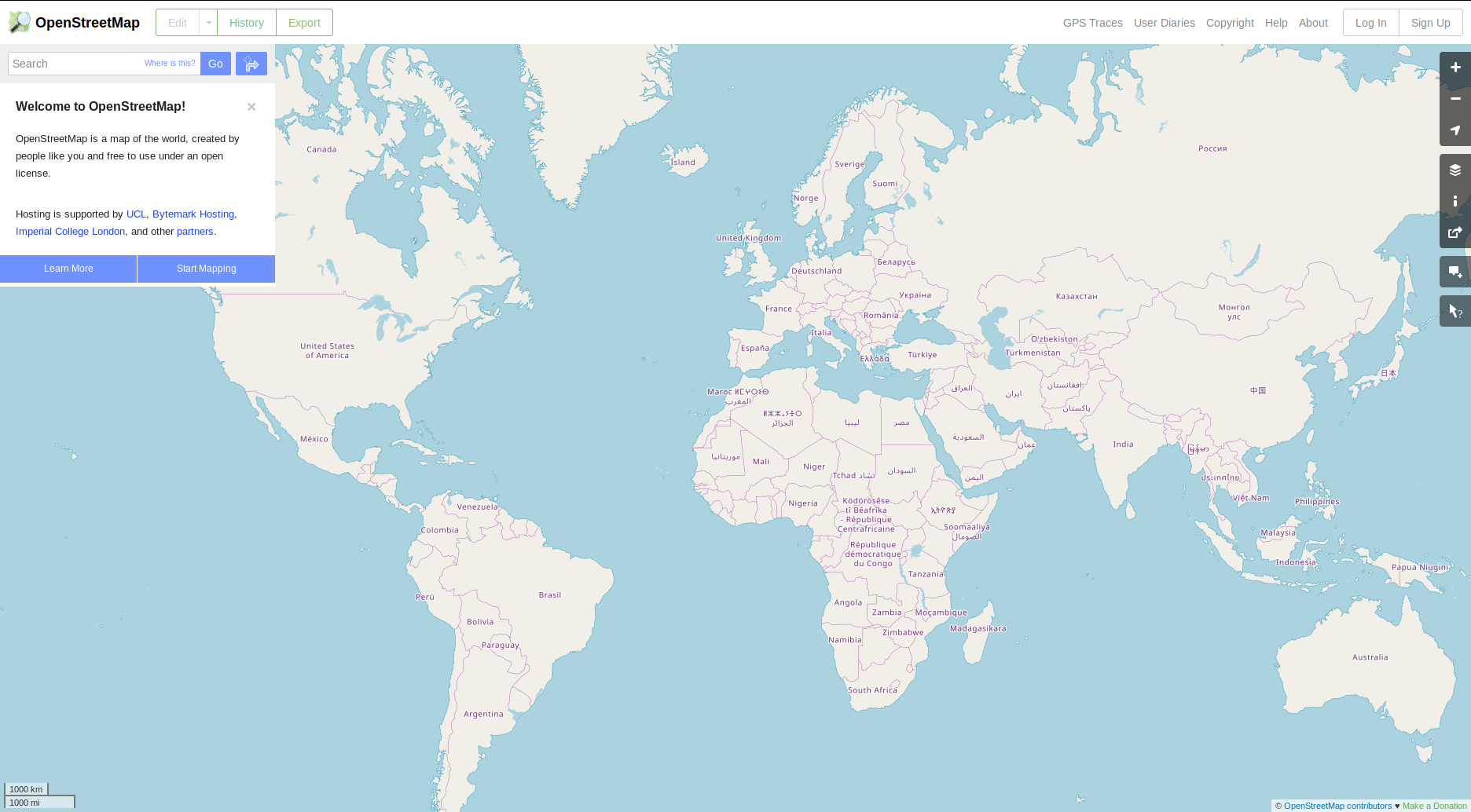
Plotly:
fig = px.scatter_mapbox(gps_data, lat="lat", lon="lon", color='direction', zoom=17, height=600)
fig.update_layout(mapbox_accesstoken=mapbox_token, mapbox_style='streets')
fig.show()
3.2.2
:
- GPS, WGS 84 .
- .
Web Mercator, — , , .
, . — , — (UTM).
Web-Mercator
UTM
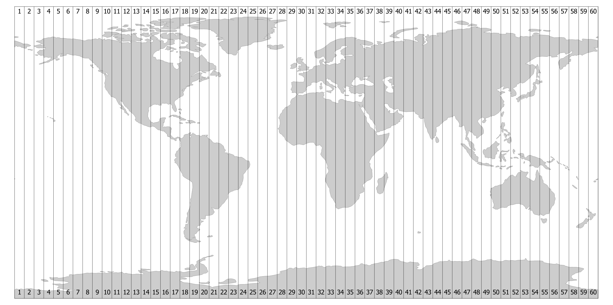
UTM Python https://github.com/Turbo87/utm, .
gps_data['xs'] = gps_data[['lat', 'lon']].apply(lambda x: utm.from_latlon(x[0], x[1])[0], axis=1)
gps_data['ys'] = gps_data[['lat', 'lon']].apply(lambda x: utm.from_latlon(x[0], x[1])[1], axis=1)
gps_data['speed_kmh'] = gps_data.speed / 1000 * 60 * 60
50 :
#
lat0 = 56.35205
lon0 = 37.51792
xc, yc, _, _ = utm.from_latlon(lat0, lon0)

r = 50
gps_data = gps_data.query(f'{xc - r} < xs & xs < {xc + r}')\
                   .query(f'{yc - r} < ys & ys < {yc + r}')
fig = px.scatter_mapbox(gps_data, lat="lat", lon="lon", color='direction', zoom=17, height=600)
fig.update_layout(mapbox_accesstoken=mapbox_token, mapbox_style='streets')
fig.show()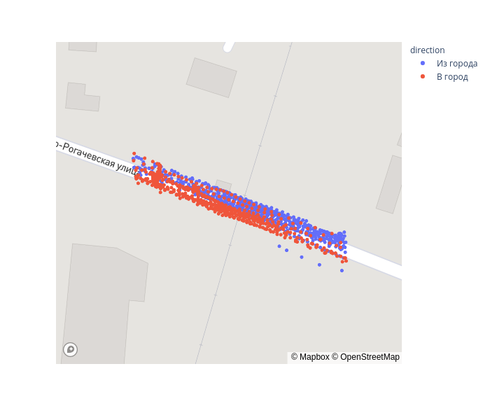
. 2d 1d, (PCA).
2 — scikit-learn. Sklearn:
pca = PCA(n_components=1).fit(gps_data[['xs', 'ys']])
gps_data['xs_transform'] = pca.transform(gps_data[['xs', 'ys']])sns.relplot(x='xs_transform', y='speed_kmh', data=gps_data, aspect=2.5, hue='direction');
. — [-5, 25]. .
accel_data['xs'] = accel_data[['lat', 'lon']].apply(lambda x: utm.from_latlon(x[0], x[1])[0], axis=1)
accel_data['ys'] = accel_data[['lat', 'lon']].apply(lambda x: utm.from_latlon(x[0], x[1])[1], axis=1)
accel_data = accel_data.query(f'{xc - r} < xs & xs < {xc + r}')\
                       .query(f'{yc - r} < ys & ys < {yc + r}')
accel_data['xs_transform'] = pca.transform(accel_data[['xs', 'ys']])
Android :
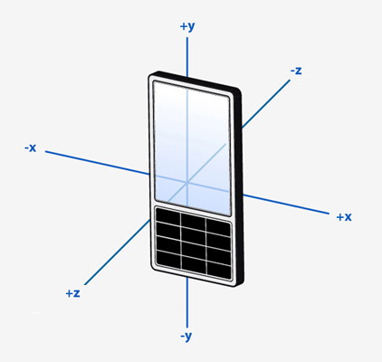
( Y). :
sns.relplot(x='xs_transform', y='ax', data=accel_data, aspect=2.5, hue='direction');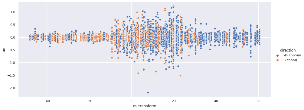
sns.relplot(x='xs_transform', y='ay', data=accel_data, aspect=2.5, hue='direction');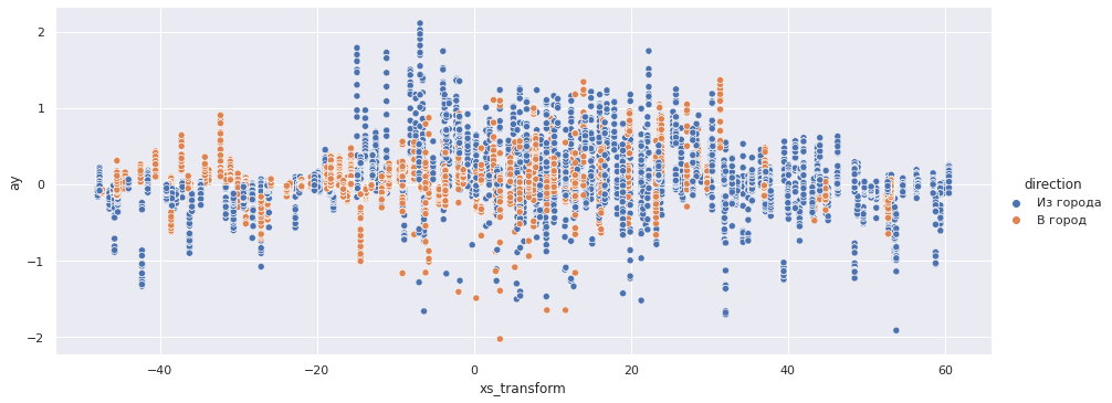
sns.relplot(x='xs_transform', y='az', data=accel_data, aspect=2.5, hue='direction');
Z:
sns.relplot(x='xs_transform', y='az', data=accel_data.query('-20 < xs_transform < 40'), aspect=2.5, hue='direction');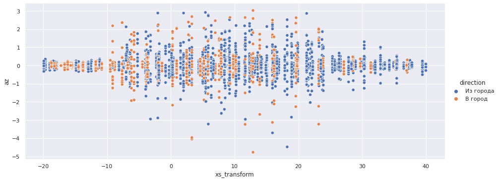
X Z — [-10, 25] 7.5.
cross = gps_data.query('-10 < xs_transform < 25')fig = px.scatter_mapbox(cross, lat="lat", lon="lon", color='direction', zoom=19, height=600)
fig.update_layout(mapbox_accesstoken=mapbox_token, mapbox_style='streets')
fig.show()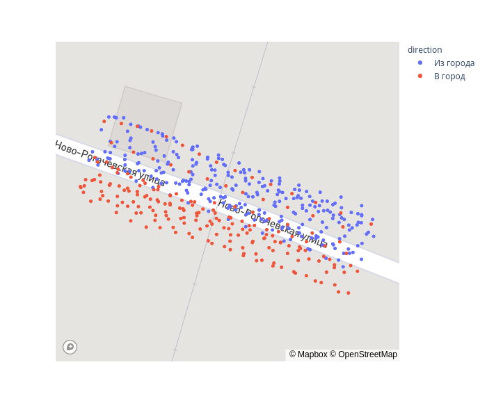
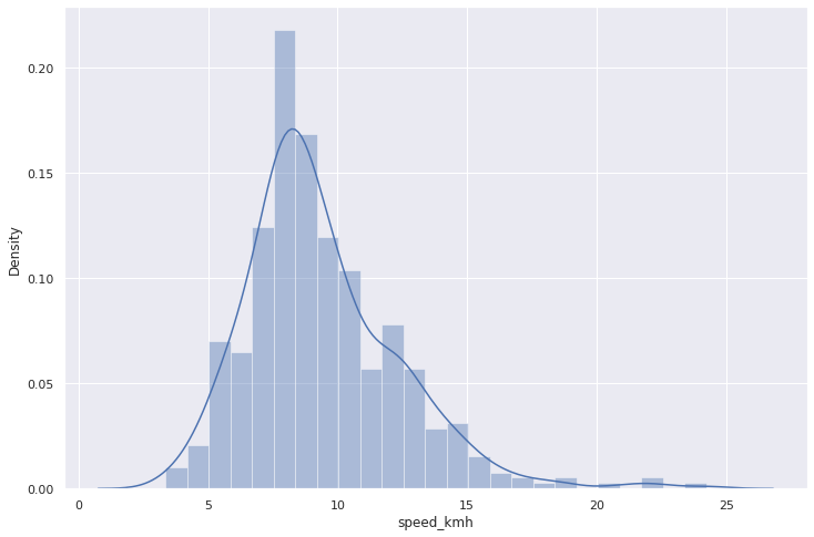
:
mean_v = cross.speed_kmh.mean()
print(f"    - {mean_v:.2} /")
sns.distplot(cross.speed_kmh);
— 9.4 /
:
base = 1
gps_data['xs_transform_round'] = gps_data['xs_transform'].apply(lambda x: base * round(x / base))
accel_data['xs_transform_round'] = accel_data['xs_transform'].apply(lambda x: base * round(x / base))sns.relplot(x='xs_transform_round', y='speed_kmh', data=gps_data, kind="line", aspect=2.5);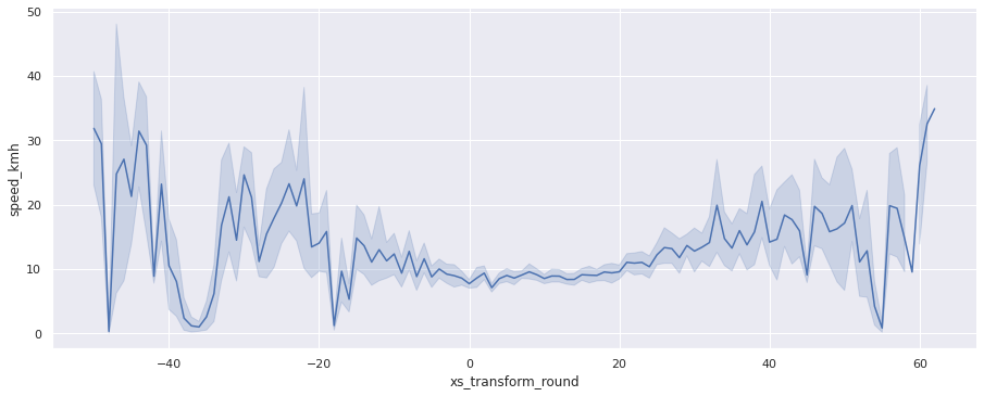
sns.relplot(x='xs_transform_round', y='az', data=accel_data, kind="line", aspect=2.5);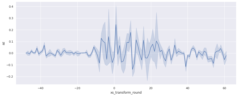
3.3
:
gps_data['flow_Tanaka'] = density_Tanaka(gps_data.speed_kmh) * gps_data.speed_kmh
gps_data['flow_Grindshilds'] = density_Grindshilds(gps_data.speed_kmh) * gps_data.speed_kmhsns.relplot(x='xs_transform_round', y='flow_Grindshilds', data=gps_data, aspect=2.5, kind='line', hue='direction');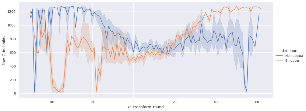
cross = gps_data.query('-10 < xs_transform < 25')mean_flow_Tanaka = cross.flow_Tanaka.mean()
print(f" - {mean_flow_Tanaka:.1f} / \
{mean_flow_Tanaka / 60:.1f} /")— 1275.5 / 21.3 /
mean_flow_Grindshilds = cross.flow_Grindshilds.mean()
print(f"      - {mean_flow_Grindshilds:.1f} / \
 {mean_flow_Grindshilds / 60:.1f} /")
— 660.0 / 11.0 /
, 700 ./.
plt.plot(V1, density_Grindshilds(V1)*V1, label=" ")
plt.xlabel(r' $V$, /')
plt.ylabel(r' $Q$, /')
plt.show()
, - 30 / — .
, :
" / ".
4.
, 10 /, .
.