It often happens when there are a lot of conversions, their price is acceptable, and sales do not grow and even fall. Here analytics "before profit per click" are no longer enough to find out the reason. And then the analysis "before the profit from the manager" comes to the rescue. Because no matter how ideally the advertising is set up, customers first interact with managers, and only then make a decision. The success of your business depends on the quality of your employees' work.
Traditional analytics systems use CRM to record the fact of a sale / contact with a manager. However, this approach only partially solves the problem: it evaluates the employee's efficiency "in the bottom line". That is, it shows sales and conversion, but leaves the communication with the client “overboard”. But the result depends on the level of communication.
To fill the gap, we have developed a tool that will automatically link each call to the manager who handled it. You don't have to use CRM and third-party services. In fact, our system puts a tag "manager's name" on every incoming call.
So the heads of the sales / customer service department will control the quality of work, find problem areas and build analytics. Fast segmentation of calls to those managers who receive them will help in this.
Formulation of the problem
The task we set ourselves is as follows: let the system know the speech patterns of all managers who can receive calls. Then for a new call you need to tag the manager, whose voice is the most "similar" in the conversation from the list of known ones.
In this case, it is considered a priori that the new phone call is successful. That is, the conversation between the manager and the client actually took place. Informally speaking, this task can be attributed to the class of tasks of "teaching with a teacher", that is, classification.
As objects - in some way vectorized (digitized) audio recordings, where only the voice of the manager sounds. The responses are class labels (manager names). Then the task of the tagging algorithm is:
- Extraction of meaningful features from audio files
- Choosing the most suitable classification algorithm
- Learning the algorithm and saving manager models
- Evaluating the quality of the algorithm and modifying its parameters
- Tagging (classifying) new calls
Some of these tasks fall into separate sub-tasks. This is due to the specifics of the conditions in which the algorithm must operate. Phone calls are usually noisy. A client within one conversation can communicate with several managers. Also, it will not take place at all, and calls often include IVR, etc.
For example, the task of tagging new calls can be divided into:
- Checking the call for success (the fact that there is a call)
- Splitting stereo into mono tracks
- Noise filtering
- Identification of areas with speech (filtering music and other extraneous sounds)
In the future we will talk about each such subtask separately. In the meantime, we will formulate the technical constraints that we impose on the input data, the resulting solution, as well as on the classification algorithm itself.
Solution constraints
The need for restrictions is partly dictated by the technique and requirements of the complexity of implementation, and also by the balance between the universality of the algorithm and the accuracy of its operation.
Limitations on the input file and training sample files:
- Format - wav or wave (you can further recode to mp3)
- The stereo must subsequently be divided into 2 tracks - the operator and the client
- Sampling rate - 16,000 Hz and above
- Bit depth - from 16 bits and more
- The file for training the model must be at least 30 seconds long and contain only the voice of a specific manager
- , , ,
All the above requirements except for the last one were formulated as a result of a series of experiments that were carried out at the stage of setting up the algorithms. This combination has shown itself to be the most effective in terms of minimizing the probability of error, namely, misclassification under easy tuning conditions.
For example, it is obvious that the longer the file in the training set, the more accurate the classifier will be. But the more difficult it is to find such a file in the call log (our training sample). Therefore, the duration of 30 seconds is a compromise between accuracy and complexity of settings. The last requirement (success) is necessary. The system should not tag a manager to a call where there was actually no conversation.
The limitations of the algorithm led to the following solution:
- , . « ». . - , .
- . , , .
The first requirement came from experimentation. Then it turned out that the "unknown" manager complicates the architecture of the solution. For this it is necessary to select thresholds after which the employee will be classified as “unrecognized”. Also, the "unknown" manager reduces accuracy by 10 percentage points.
In addition, an error of the second kind appears when a known manager is classified as unknown. The probability of such an error is 7-10%, depending on the number of known ones. This requirement can be called essential. It obliges the algorithm tuner to indicate all managers in the training sample. And also introduce models of new employees there and remove those who quit.
The second requirement stems from practical considerations and the architecture of the algorithm we are using. In short, the algorithm splits the analyzed audio into speech fragments and "compares" each one with all the trained manager models one by one.
As a result, a "mini-tag" is assigned to each of the mini-fragments. With this approach, there is a high probability that some of the fragments are recognized incorrectly. For example, if they remain noisy or their length is too short.
Then, if all the "mini-tags" are displayed in the final solution, then in addition to the tag of the real manager, a lot of "trash" ones will be displayed. Therefore, only the most "frequent" tag is displayed.
Description of input / output data
We will divide the input data into 2 types:
Data at the input of the algorithm for generating models of managers (data for training):
- Audio file + class label
Data at the input of the tagging algorithm (data for testing / normal operation):
- External data (audio file)
- Internal data (saved models)
The output is also divided into 2 types:
- Output data of the model generation algorithm
- Trained manager models
- Output from the tagging algorithm
- Manager tag
At the input of the algorithm in any mode of its operation, an audio file that meets the requirements is received. They are in the "restrictions" section.
At the input of the model generation algorithm, it is allowed that several input files correspond to one class (manager). But one file cannot correspond to multiple managers. The class label name can be placed in the file name. Or just create a separate directory for each employee.
The input-based model training algorithm generates many models that can be loaded during training. Their number corresponds to the number of different tags in the set of audio files.
Thus, if there are M files that are marked with n different class labels, the algorithm creates n models of managers at the training stage:
- Model_manager_1.pkl
- Model_manager_2.pkl
- ...
- Model_manager_n.pkl
where instead of " manager _... " is the name of the class.
The input to the tagging algorithm is an unlabeled audio file, in which a priori there is a conversation between a manager and a client, as well as n employee models. As a result, the algorithm returns a tag - the name of the class of the most "plausible" manager.
Data preprocessing
Audio files are pre-processed. It is sequential and runs both in tagging mode and in model training mode:
- Checking the success of the call - only at the tagging stage
- Splitting stereo into 2 mono tracks and further work only with the operator's track
- Digitization - extraction of audio signal parameters
- Noise filtering
- Removing "long" pauses - identifying fragments with sound
- Filtering for non-speech fragments - removing music, background, etc.
- Fusion of fragments with speech (only at the stage of training)
We will not dwell on the success check stage. This is a subject for a separate article. In short, the essence of the stage is that the call is classified according to whether there is a conversation of "living people" in it. By “living people” we mean a client and a manager, not a voice assistant, music, etc.
The success of a call is checked using a specially trained classifier with an external threshold - “the minimum duration of a conversation after which the call is considered successful”.
At the second stage, the stereo file is divided into 2 tracks: the manager and the client. Further processing is carried out only for the employee's track.
At the stage of digitization, the parameters of the "feature" are extracted from the operator track, which are a digital representation of the signal. We at Calltouch used chalk-cepstral components. In addition, the parameters are extracted on a very small fragment, which is called the window width (0.025 seconds). All features are normalized at the same time.
nfft=2048 //
appendEnergy = False

def get_MFCC(sr,audio): //    , sr=16000 -
features = mfcc.mfcc(audio, sr, 0.025, 0.01, 13, 26, nfft, 0, 1000,  appendEnergy)
    features = preprocessing.scale(features)
    return features

count = 1
features = np.asarray(()) //
for path in file_paths: //
path = path.strip()
sr,audio = read(source + path) //
vector = get_MFCC (sr, audio) #
if features.size == 0:
     features = vector
else:
     features = np.vstack((features, vector))
At the output, each audio file turns into an array, in which the mel-cepstral characteristics of each 0.025 second fragment are recorded line by line.
Further processing of the file consists in filtering noise, removing long pauses (not pauses between sounds), and searching for speech. These tasks can be accomplished using various tools. In our solution, we used methods from the pyaudioanalysis library:
clear_noise(fname,outname,ch_n) # .- fname - input file
- outname - output file
- ch_n - number of channels
At the output, we get the file outname, which contains the sound, cleaned from noise, from the file fname.
silenceRemoval(x, Fs, stWin, stStep) # « »- x - input array (digitized signal)
- Fs - sampling rate
- stWin - width of the feature extraction window
- stStep - offset step size
At the output, we get an array of the form:
[l_1, r_1]
[l_2, r_2]
[l_3, r_3]
…
[l_N, r_N]
where l_i is the start time of the i-th segment (sec), r_i is the end time of the i-th segment (sec ).
detect_audio_segment(x,thrs) # .- x - input array (digitized signal)
- hrs - minimum length (in seconds) of the detected speech fragment
At the output, we get those fragments [l_i, r_i] that contain speech lasting from thrs seconds.
As a result of preprocessing, the input audio file is converted to the form of an array:
[l_1, r_1]
[l_2, r_2]
[l_3, r_3]
…
[l_N, r_N],
where each fragment is a time interval of the cleaned speech file.
Thus, we can match each such fragment with a matrix of features (small-cepstral characteristics), which will be used for training the model and at the tagging stage.
Methods / Algorithms Used
As noted above, our solution is based on the pyaudioanalysis.py library written in Python 2.7. In view of the fact that our general solution is implemented in Python 3.7, some of the library functions have been modified and adapted for this version of the language.
In general, the algorithm of the tool for tagging managers can be divided into 2 parts:
- Model manager training
- Tagging
A more detailed description of each part looks like this.
Model manager training:
- Loading the training sample
- Data preprocessing
- Counting the number of classes
- Creating a manager model for each of the classes
- Saving the model
Tagging:
- Call loading
- Checking the call for success
- Pre-processing a successful call
- Loading all trained manager models
- Classification of each fragment of the processed call
- Finding the most likely manager model
- Tagging
We have already discussed in detail the tasks of data preprocessing. Now let's look at methods for creating manager models.
We used the GMM (Gaussian Mixture Model) algorithm as a model . He models our data under the assumption that they are realizations of a random variable with a distribution that is described by a mixture of Gaussians - each with its own variance and its own mathematical expectation.
It is known that the most common algorithm for finding the optimal parameters of such a mixture is the EM (Expectation Maximization) algorithm . He divides the difficult problem of maximizing the likelihood of a multidimensional random variable into a series of maximization problems of lower dimension.
As a result of a series of experiments, we came to the following parameters of the GMM algorithm:
gmm = GMM(n_components = 16, n_iter = 200, covariance_type='diag',n_init = 3)Such a model is created for each manager, and then it is trained - its parameters are adjusted to specific data.
gmm.fit(features)Next, the model is saved to be used at the tagging stage:
picklefile = path[path.find('/')+1:path.find('.')]+".gmm"
pickle.dump(gmm,open(dest + picklefile,'wb'))
At the tagging stage, we load the previously saved models:
gmm_files = [os.path.join(modelpath,fname) for fname in
                  os.listdir(modelpath) if fname.endswith('.gmm')]
modelpath is the directory where we saved the models.
models = [pickle.load(open(fname,'rb'),encoding='latin1') for fname in gmm_files]And also load the names of the models (these are our tags):
speakers   = [fname.split("/")[-1].split(".gmm")[0] for fname
                  in gmm_files]
The uploaded audio file, for which you need to tag, is vectorized and preprocessed. Further, each fragment with the speech in it is compared with the trained models and the winner is determined in terms of the maximum logarithm of likelihood:
log_likelihood = np.zeros(len(models)) #

for i in range(len(models)):
            gmm    = models[i]  #
            scores = np.array(gmm.score(vector))
            log_likelihood[i] = scores.sum() #  i  –

winner = np.argmax(log_likelihood) #
print("\tdetected as - ", speakers[winner])
As a result, our algorithm has approximately the following conclusion:
starts in: 1.92 ends in: 8.72
[-10400.93604115 -12111.38278205]
detected as - Olga
starts in: 9.22 ends in: 15.72
[-10193.80504138 -11911.11095894]
detected as - Olga
starts in: 26.7 ends in: 29.82
[-4867.97641331 -5506.44233563]
detected as - Ivan
starts in: 33.34 ends in: 47.14
[-21143.02629011 -24796.44582627]
detected as - Ivan
starts in: 52.56 ends in: 59.24
[-10916.83282132 -12124.26855 starts538]
detected as - Olga
starts538 in: 116.32 ends in: 134.56
[-36764.94876054 -34810.38959083]
detected as - Olga
starts in: 151.18 ends in: 154.86
[-8041.33666572 -6859.14253903]
detected as - Olga
starts in: 159.7 ends in: 162.92
[-6421.72235531 -5983.90538059]
detected as - Olga
starts in: 185.02 ends in: 208.7
…
starts in: 442.04 ends in: 445.5
[-7451.0289772 -6286.6619 ]
detected as - Olga
*******
WINNER - Olga
This example assumes that there are at least 2 classes - [Olga, Ivan] . The audio file is cut into segments [1.92, 8.72], [9.22, 15.72],…, [442.04, 445.5] and the most suitable model is determined for each of the segments.
The cumulative likelihood logarithm is shown in parentheses next to each chunk:[-10400.93604115 -12111.38278205] , the first element is Olga's likelihood and the second is Ivan . Since the first argument is greater than the second, this segment is classified as Olga . The final winner is determined by the majority of the "votes" of the fragments.
results
Initially, we designed the algorithm on the assumption that an “unknown” manager may be present in incoming calls - that is, such that his model is not present in the training sample.
To detect such a user, we need to enter some metric on the log_likelihood vector . Such that certain of its values will indicate that most likely this fragment is not adequately described by any of the existing models. We suggested the following metric as a test:
Leukl=(log_likelihood-np.min(log_likelihood))/(np.max(log_likelihood)-np.min(log_likelihood))
-sorted(-np.array(Leukl))[1]<T
This value indicates how “evenly” the scores are distributed in the log_likelihood vector . The uniformity of estimates (their proximity to each other) means that all models behave in the same way and there is no clear leader.
This suggests that most likely all models are wrong and we have a manager who was not at the training stage. The relationship between T and the quality of the classification is shown in the figures.
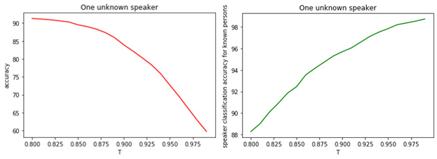
Figure: 1.
a) The accuracy of the binary classification of known and unknown managers.
b) The accuracy of the classification of famous managers.

Figure: 2.
a) The proportion of well-known managers assigned to the class of well-known managers.
b) The proportion of unknown managers assigned to the class of known.
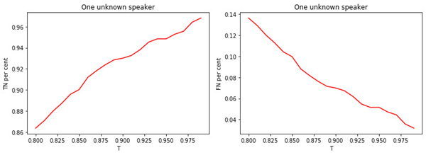
Figure: 3.
a) The share of unknown managers assigned to the class of unknowns.
b) The proportion of well-known managers assigned to the class of unknowns.
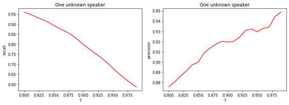
Figure: 4.
a) Completeness of the binary classification (recall).
b) Precision of binary classification (precision).
The relationship between the value of the threshold T and the quality of classification (tagging) is obvious. The larger T (the stricter the conditions for assigning a manager to the class of unknowns), the less likely a well-known manager to be classified as unknown. But it is more likely to "miss" an unknown manager.
The optimal threshold value is 0.8 . Because we classify well-known managers with an accuracy of about 90%and determine the "unknowns" with an accuracy of 81% . If we assume that all managers are "familiar" to us, then the accuracy will be about 98% .
conclusions
In the article, we described the general ideas of the functioning of our tool for identifying managers in calls. Of course, we do not pretend that our algorithm is optimal and not capable of improving.
It is based on a number of assumptions that are not always met in practice. For example, we may encounter an unknown manager if there is no data about him. Or, two or more managers can conduct a conversation with a client "in equal shares." From the point of view of the algorithm, the following directions for further improvements can be proposed:
- Choosing a different algorithm model than GMM
- Optimizing GMM parameters
- Selecting a different metric for detecting a new manager
- Search for the most significant features of the speech signal
- Combination of different audio preprocessing tools and optimization of parameters of these methods