🍍 🎃 👩🏾‍🔧 Making decisions. Example 📁 🌯 👩🏽‍🚒

Other articles in the cycle

Continuing the topic, I will say that I looked at the publications of other Habr authors on this topic. There is interest in problems, but no one wants to get into theory. Acting like pioneer discoverers. It would be great if they receive new results, achievements, but no one strives for this.

But in fact, it turns out worse than it is already known, a lot of factors are not taken into account, the results of the theory are used where it does not recommend doing it and in general everything does not look very serious, although Habr, as it should be understood, does not strive for this. Readers cannot and should not act as a filter.

The original set of alternatives, their measurement and evaluation

It is known that the problems of finding a solution arise only in multi-alternative situations of choice. To consider the decision-making situation, formulate a specific decision-making problem (DP), choose a method for solving it, it is necessary to have some initial information about alternatives, a preference relation.

Let us show in the subsection what methods of obtaining it exist. Alternatives have many properties (features) that influence the decision. For example, indicators of properties of objects (weight, volume, hardness, temperature, etc.) can be quantitative or qualitative.

Let some property of the set of alternatives from Ω be expressed by a number, that is, there exists a mapping ψ: Ω → E1, where E1 is the set of real numbers. Then this property is characterized by an indicator, and the number z = ψ (x) is called the value (estimate) of the alternative in terms of the indicator.

To evaluate alternatives, it is necessary to measure the indicators.

Definition. The measurement of an indicator of a certain property is understood as assigning numerical values to individual levels of this indicator in certain units. In this case, the choice of the unit of measurement is important.

So, for example, if the volume of a certain part of the container is first measured in cubic meters and then in liters, then the essence of the indicator will not change; only the number of units will change. These property metrics can be scaled, multiplied, or divided by a constant value for the property metric.

On the other hand, there are properties whose indicators do not allow such manipulation of their values. The degree of heating of bodies is characterized by temperature and is measured in degrees. The value of this indicator + 10 ° and –15 ° does not allow to judge how many times the body with a temperature of + 10 ° is heated more than a body with a temperature of –15 °

From these examples, it is possible (and important) to conclude that the indices volume and temperature refer to different types of properties, over the values of z = ψ (x) of which certain transformations f (z) = f (ψ (x)) are admissible or impermissible ...

Namely, the set of admissible transformations f (z) is taken as the basis for determining the type of the scale in which the indicator of a certain attribute (property) is measured. Performing one or another measurement of the indicator of a feature that is highlighted by the researcher, we come to the task of determining the type of scale in which the measurement should be carried out.

Without solving this problem correctly, we can admit incorrect handling of the results of observations (measurements) when processing them. This happens when the values of the indicators undergo transformations taken outside the set of transformations allowed for a given type of scale.

Definition. A measurement scale is a sequence of values of the same name of various sizes accepted by agreement.

Let's consider in more detail the main types of scales.

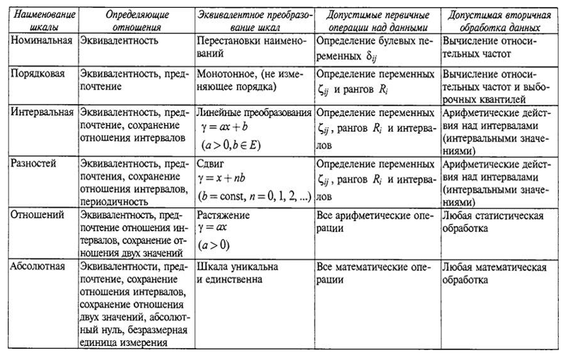
1. Nominal scales . Nominal scales are used when a researcher deals with objects described by some characteristics. Depending on whether a given object has a certain value of a feature or its absence, the object is referred to one or another class.

For example, if we are talking about people, then the value of the feature (the scale of the feature is formed by two values of sex: male and female) makes it possible to unambiguously assign each person to a certain class. For this reason, the scale is called the grading scale. Such a sign as a profession allows a person to be called, for example, a teacher, a carpenter, or otherwise in accordance with the value of the indicator of the profession.

The scale in this case is formed by the names of all professions. Obviously, on this scale, zero is not indicated, although the absence of a profession in the subject allows him to be assigned precisely to the category of people without a profession. The names of the professions are not ordered in any way on this scale, although they are often arranged alphabetically for reasons of convenience.

From these considerations, such a scale is called the naming scale.

Valid transformations of values in this scale are all one-to-one functions: f (x) ≠ f (y) <=> x ≠ y.

2. Ordinal scales . If the studied trait, for example, the hardness of the material, manifests itself differently in objects and has values that cannot be specifically measured, but one can unequivocally judge the comparative intensity of its manifestation for any two objects, then they say that the value of the trait is measured on an ordinal scale. A classic example of this is the hardness of minerals. The reference point is 0 on the scale is not defined.

The characteristic value is defined as follows. The harder mineral of the pair in question leaves a scratch on the other. All minerals according to the values of this trait can be ordered as follows: the first is the least hard, the second is harder, it leaves a scratch only on the first, the third leaves a scratch on the first two, etc.

The difference between the ordinal scale and the nominal is that the values of the trait can be sorted out, while the values on the nominal scale cannot even be ordered. The disadvantage of an ordinal scale is that it is not proportional.

It is impossible to answer the question of how much or how many times one mineral is harder than another. The admissible transformations of the ordinal scale consist of all monotonically increasing functions with the property: x ≥ y => f (x) ≥ f (y).

3.Interval scale (interval). differ from the scales of order in that for the properties they describe, it makes sense not only the equivalence and order relations, but also the summation of intervals (differences) between various quantitative manifestations of properties. A typical example is the time interval scale.

Time intervals (for example, work periods, study periods) can be added and subtracted, but adding the dates of any events is meaningless.

Another example, the scale of lengths (distances) - spatial intervals is determined by aligning the zero of the ruler with one point, and the reading is done at another point. This type of scale also includes the temperature scales Celsius, Fahrenheit, Reaumur.

Linear transformations are admissible in these scales, (x - y) / (z -v); x ∓ y; they apply procedures to find the mathematical expectation, standard deviation, asymmetry coefficient, and displaced moments.

4. Scale of differences (point) Scales of differences differ from scales of order in that according to the scale of intervals it is possible to judge not only that the size is larger than another, but also how much more, in essence, this is the same absolute scale, but its values are shifted by some value relative to the absolute values (x - y) <(z -v); x ∓ y;

5. Relationship scale... The scale for which the set of admissible transformations consists of all similarity transformations is called the scale of relations. The reference point is fixed on this scale and the measurement scale can be changed for it.

Let this scale measure the length of an object. In this case, you can switch from measuring in meters to measuring in centimeters, decreasing the unit of measurement by a factor of 100. Obviously, in this case, the ratio of the lengths L (A) and L (B) of two objects A and B, measured in the same units, will not change when the units are changed.

The values of the indicator of the trait, measured in this scale, allow you to

answer the question how many times more intensely the trait manifests itself in one object than in another. For this purpose, it is necessary to consider the ratio of the values L (A) / L (B) = k.

If the ratio is greater than one (k> 1), the value of the feature indicator for the first object A is k times greater than that for B, if k <1, then the value of the feature indicator for object B is 1 / k times greater than that for A. is multiplication by a positive integer and only that.

6. Absolute scale . The simplest of all scales is a scale that allows only one transformation f (x) = x. This situation corresponds to the only way to measure the indicator of the property of an object, namely a simple recount of objects.

This scale is called the absolute scale. When we register object x, we are not interested in anything other than this object. The absolute scale can be considered as a particular implementation of some other scales.

Decision-making task. Getting a matrix of relations

We list the possible settings of the ZPR, these include:

linear ordering of alternatives (the top in the chain is the best);
highlighting the best alternative;
highlighting a (unordered) subset of the best alternatives;
highlighting an ordered subset of the best alternatives;
partial ordering of alternatives;
ordered (partially ordered) splitting of alternatives;
unordered partition of alternatives (classification).

Based on the analysis of measurements of indicators of properties of alternatives in different scales, the measurement results can be presented in different ways [1, 5].

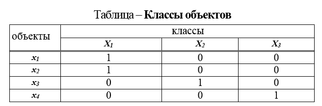
1. Classification table. The table is obtained when measurements are taken in nominal scales and is a table, the rows of which are: the name of the object, and the columns are the names of the classes

X_{1}, X_{2}, X_{3},

$X_1, X_2, X_3,$ ... etc. In the columns class 1, class 2, etc., 1 is put if the object belongs to this class and 0 - if not (Table Classes of objects).

In the class table, objects

x_{1}, x_{2} є X_{1}, x_{3} є X_{2}, x_{4} є X_{3} .

$x_1 ,x_2 є X_1, x_3 є X_2, x_4 є X_3.$

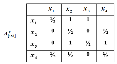
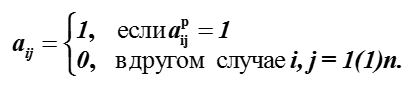
2. Matrix of preference relations. Obtained by taking measurements in ordinal scales. To reveal preferences on the set of objects Ω means to indicate the set of all those pairs of objects (x, y) from this set for which the object x is preferable (for example, harder) than the object y. The preference relationship matrix is obtained as follows. (see here, fig 2.15)

Under construction

А_{[n \times n]}^{p}

$_{[n×n]}^p$ square matrix. Its i-th line corresponds to the i-th element

x_{i}

$x_i$ set Ω, and the jth column to the element

x_{j}

$x_j$ . At the intersection of the i-th row and the j-th column, 1 is placed if the object

x_{i}

$x_i$ preferred over object

x_{j}

$x_j$ , zero if the object

x_{j}

$x_j$ preferred over object

x_{i}

$x_i$ , 1/2 if objects

x_{i}

$x_i$ and

x_{j}

$x_j$ indifferent, and nothing is put - if the objects are incomparable

x_{i}

$x_i$ and

x_{j}

$x_j$ cannot be compared.

An example of such a preference relationship is presented in the matrix below.

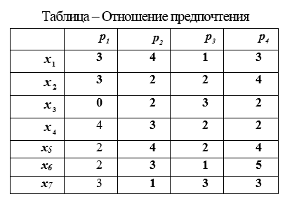
3. Table of indicators. Obtained when measuring in the scale of relations. The properties of the indicators that will be measured are selected. The measurement of these properties is performed, and the measurement results are recorded in a table.

In columns

p_{1}, p_{2}, p_{3}, p_{4}

$p_1, p_2, p_3, p_4$ tables Preference ratio contains the values of property indicators by which objects are evaluated

x_{1}, x_{2}, x_{3}, x_{4}, x_{5}, x_{6}

$x_1,x_2,x_3,x_4,x_5,x_6$ and

x_{7}

$x_7$ .

After receiving the measurement results in these forms of presentation, we need to display the results in the form of relations, since we will solve the ZPR, relying on the well-developed apparatus of the theory of binary relations.

The mapping of the preference table to the binary relation matrix is as follows:

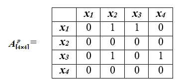
From the preference relationship matrix

for 4 alternatives presented in table. The preference relationship will be the matrix

А_{[4 \times 4]}^{p}

$_{[4×4]}^p$

, which looks like this:

А_{[4 \times 4]}^{p}

$_{[4×4]}^p$

The mapping of the scorecard to the preference ratio matrix is as follows:

a_{i, j} = 1

$a_{i,j}=1$ if:

1) the number of indicators by which the object

x_{i}

$x_i$ preferred over object

x_{j}

$x_j$ greater than the number of indicators by which the object

x_{j}

$x_j$ preferred over object

x_{i}

$x_i$ ;

2) for the object

x_{i}

$x_i$ none of the indicators takes the smallest possible value.

3) condition 1 implies that those indicators for which the object

x_{i}

$x_i$ not worse than object

x_{j}

$x_j$ , make up the majority of all the indicators under consideration.

However, if this condition is met, it may turn out that according to those indicators for which the object

x_{i}

$x_i$ worse than object

x_{j}

$x_j$ , the difference is significant; To reduce the number of such cases when giving preference to x, condition 2 is introduced.

Methods for solving the problem of decision making

Let, after receiving the initial data, we have the relation R on the set of alternatives

Ω = (x_{1}, . . ., x_{n})

$Ω= {(x_1, ...,x_n)}$ ... And the task is to make a decision. The main method is linear ordering (ranking) of alternatives, that is, building alternatives in a chain in descending order of their value, suitability, importance, and the like, from the “best” to the “worst”.

The ratio R can be:

complete non-transitive attitude;
a partial order relation;
linear order.

Only in the case of linearity of the relation R, the structure of preferences meets the task. In this case, the ranking of alternatives from the set Ω is obtained directly by constructing a line diagram of the ordered set. In the diagram, the alternative

x_{i}

$x_i$ , will be strictly higher than the alternative

x_{j}

$x_j$ if preferred.

The solution of the problem posed for complete and transitive relations is carried out using methods (algorithm) for ranking alternatives, and for partial orders using a linear reordering algorithm. These algorithms will be discussed in the following paragraphs below.

Ranking of alternatives . Let the relation [Ω, R] be complete and nontransitive. The completeness property means that all alternatives

Ω = (x_{1}, . . ., x_{n})

$Ω = {(x_1, ...,x_n)}$ from the set are comparable to each other. The presence of nontransitivity is possible only if the preference graph G [Ω, R] contains contours.

It is necessary to transform the structure of the relationship graph so that logical contradictions in the form of contours are eliminated. If we assume that there is a contour in relation to R

x_{1}, x_{2}, \dots, x_{k}, x_{1},

$x_1, x_2, …,x_k, x_1,$ then when ranking alternatives

x_{1}

$x_1$ should be located higher

x_{2}, x_{3}, \dots, x_{k}, x_{1},

$x_2, x_3, …,x_k, x_1,$ , which leads to a contradiction.

Let us introduce the following statement [1,5].

Let B 'and B "be two arbitrary contours of a graph of the form G [Ω, R], then if some element

x_{i}

$x_i$ є B 'dominates element

x_{j}

$x_j$ є B '', then any element

x_{1}

$x_1$ є B 'any element dominates

x_{k}

$x_k$ є B ''.

This proposal makes it possible to partition the set R into m subsets

B_{1}, B_{2}, \dots, B_{m}

$B_1, B_2, …,B_m$ such that

B_{i} \cap B_{j} = \emptyset, \forall i, j є [1, m]; U B_{i} = Ω .

$B_i ∩ B_j=∅, ∀i,j є [1, m]; UB_i =Ω.$

So, the problem of ranking the alternatives of the set falls into two stages:

1) the selection of the contours of the graph, i.e. partition of the set Ω into subsets

B_{1}, B_{2}, \dots, B_{m}

$B_1, B_2, …,B_m$ and the group ordering of these subsets;

2) ranking of the contour elements selected at the first stage.

Algorithm for highlighting the contours of a graph

To find the contours of a graph, there is a simple algorithm [1]. Let be

А_{[n \times n]}

$_{[n×n]}$ Is the adjacency matrix of the graph G [Ω, R], and

Е_{[n \times n]}

$_{[n×n]}$ –Unit matrix. We form

Е_{[n \times n]} + А_{[n \times n]}

$_{[n×n]}+ _{[n×n]}$ ,

(Е_{[n \times n]} + А_{[n \times n]})^{2}

$(_{[n×n]}+ _{[n×n]})^2$ ,

(Е_{[n \times n]} + А_{[n \times n]})^{3}

$(_{[n×n]}+ _{[n×n]})^3$ ,… A sequence of degrees of matrices, whose elements express the number of paths of length at most 1, 2, 3… For some value m ≤ n, we obtain the following equality (a steady matrix):

(Е_{[n \times n]} + А_{[n \times n]})^{m} = (Е_{[n \times n]} + А_{[n \times n]})^{m + 1}

$(_{[n×n]}+ _{[n×n]})^m=(_{[n×n]}+_{[n×n]})^{m+1}$ ...

It is known from graph theory [10] that to each system of all identical rows of a “steady” matrix there corresponds a subset of the vertices of the graph lying in one contour. Grouping the corresponding vertices into classes, we obtain a partition of the original set Ω into subsets

B_{1}, B_{2}, \dots, B_{m}

$B_1, B_2, …,B_m$ ...

Obviously, among these subsets one can find such a subset

B_{i} m

$B_im$ that the elements of this subset will not be dominated by any elements from other subsets. This subset will be considered the best, and it will take the first place in the ranking in descending order of preference.

Then we find the best subset among the remaining subsets using the same principle and put it in second place. We will

continue this procedure until all subsets take their places in the ranking.

Let the preference relation R be given on the set Ω by the matrix

А_{[6 \times 6]}

$_{[6×6]}$ ...

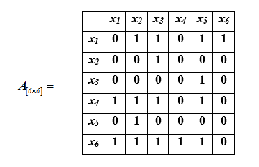
The relation graph R is shown in Fig. G.

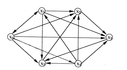
Figure: D. Graph of non-transitive relation R

To implement the first stage of ranking the elements of the set, it is necessary to select the contours of the graph G [Ω, R]. This is done by raising the adjacency matrix of the graph to successive powers until the matrices match.

We get

(Е_{[6 \times 6]} + А_{[6 \times 6]})

$(_{[6×6]}+ _{[6×6]})$ ,

(Е_{[6 \times 6]} + А_{[6 \times 6]})^{2}

$(_{[6×6]}+ _{[6×6]})^2$ ,

(Е_{[6 \times 6]} + А_{[6 \times 6]})^{3}

$(_{[6×6]}+ _{[6×6]})^3$ ...

Next, we sequentially calculate the increasing powers of the matrix, summing them with the unit matrix of the corresponding dimension until the matrix stops changing:

Because

(Е_{[6 \times 6]} + А_{[6 \times 6]})^{2} = (Е_{[6 \times 6]} + А_{[6 \times 6]})^{3}

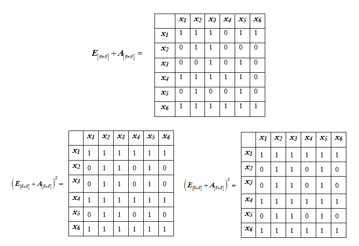
$(_{[6×6]}+ _{[6×6]})^2 =(_{[6×6]}+ _{[6×6]})^3$ , we can conclude that

(Е_{[6 \times 6]} + А_{[6 \times 6]})^{2} = (Е_{[6 \times 6]} + А_{[6 \times 6]})^{k}

$(_{[6×6]}+ _{[6×6]})^2 = (_{[6×6]}+ _{[6×6]})^k$ , for k ≥ 2. From the analysis of the matrix

(Е_{[6 \times 6]} + А_{[6 \times 6]})^{2}

$(_{[6×6]}+ _{[6×6]})^2$ it follows that the lines corresponding to the elements

x_{1}, x_{4}, x_{6}

$x_1,x_4,x_6$ coincide, this indicates that these elements belong to the same contour of the graph G [Ω, R].

The elements

x_{1}, x_{4}, x_{6}

$x_1,x_4,x_6$ form a set

B_{1} = (x_{1}, x_{4}, x_{6})

$B_1 =(x_1,x_4,x_6)$ ... Another contour is formed by elements

x_{2}, x_{3}, x_{5}

$x_2,x_3,x_5$ which are included in the set

B_{2} = (x_{2}, x_{3}, x_{5})

$B_2 =(x_2,x_3,x_5)$ ...

Thus, we have partitioned the set into m = 2 classes

B_{1}, B_{2}

$B_1, B_2$ ... Let us carry out a group ordering of these subsets. To do this, you need to find some element

x_{i} є B_{1}

$x_i є B_1$ which element dominates

x_{j} є B_{2}

$x_j є B_2$ ...

This will mean the superiority of the subset

B_{1}

$B_1$ over

B_{2}

$B_2$ ... In our example

x_{1} є B_{1}

$x_1 є B_1$ dominates

x_{2} є B_{2}

$x_2 є B_2$ ... Therefore, the subset

B_{1}

$B_1$ dominates

B_{2}

$B_2$ ... A graphical representation of dominance in the partition Ω is shown in Fig. QC.

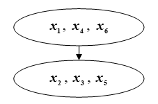
Figure: QC. Ranking of the contours selected at the first stage

Algorithm for ranking the elements of the contours . Is it possible to arrange the elements of a relation lying in the same contour, are they equivalent to each other, or are there sufficiently subtle differences between them to distinguish them? It turns out that such a possibility, as a rule, exists [1].

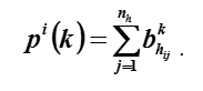
Let us denote by

B_{h_{[n \times n]}}

$B_{h_{[n×n]}}$ the adjacency matrix of the h-th contour. Let's introduce the concept

p^{i} (k)

$p^i(k)$ is the force of order k of element i, the value of which is calculated as the sum of the elements of the i-th row in the matrix

B_{h_{[n \times n]}}^{k}

$B_{h_{[n×n]}}^k$ (1).

Let be

b_{h_{[i, j]}}^{k}

$b_{h_{[i,j]}}^k$ Is the element in the i-th row and j-th column of the matrix, then

The relative strength of the k-th order of the element i is understood as the fraction

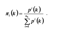
As k increases unbounded (k → ∞), the number

π_{i} (k)

$π_i(k)$ tends to a certain limit π, which we will further call the strength of the element i. Vector

П_{[n]} = (π_{1}, . . ., π_{n})

$_{[n]} = (π_1,...,π_n)$ is called the limit vector.

Due to the Perron-Frobenius theorem [1], the limit always exists. The normalized eigenvector of the contour adjacency matrix coincides with its limit vector. Therefore, the vector

П_{[n]} = (π_{1}, . . ., π_{n})

$_{[n]} = (π_1,...,π_n)$ (2)

can be found without calculating the integrated forces

p^{i} (k)

$p^i(k)$ , by solving the system of linear equations

B_{h_{[n \times n]}} \cdot П_{[n]} = λ П_{[n]}

$B_{h_{[n×n]}} · _{[n]} = λ_{[n]}$ , (3)

where λ is the largest non-negative real root of the characteristic equation

d e t (λ Е_{[n \times n]} - B_{h_{[n \times n]}}) = 0

$det(λ_{[n×n]}- B_{h_{[n×n]}}) = 0$ (4)

It should be noted that the normalized eigenvector of a nonnegative indecomposable matrix does not change when the matrix is multiplied by a number s> 0, as well as when it is summed with a matrix of the form sE.

Then the contour elements are ordered by decreasing values of the corresponding vector components

П_{[n]}

$_{[n]}$ , i.e. element i dominates element j when

π_{i} > π_{j}

$π_i >π_j$ ...

We will rank the elements of the set

B_{1} = (x_{1}, x_{4}, x_{6})

$B_1 =(x_1,x_4,x_6)$ ... Let's construct a preference matrix for this set

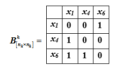
The vector of integrated forces of the 1st order for the elements

(x_{1}, x_{4}, x_{6})

$(x_1, x_4, x_6)$ looks like (1,1,2), the vector of relative forces P (k) = (1 / 4,1 / 4,2 / 4).

Item ranking

(x_{1}, x_{4}, x_{6})

$(x_1, x_4, x_6)$ the strength of the 1st order is shown in Fig. R.

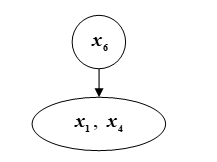
Figure: R. Ranking of elements

Let us find vectors characterizing the forces of the 2nd, 3rd, 4th and 5th orders.

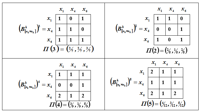
A graphical representation of the ranking is shown in Fig. P.

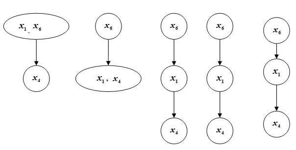
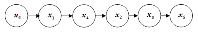
Fig. C - Chain

Carrying out the ranking of the elements of the set B2 in a similar way, we obtain the results presented in Fig. Right.

As a result of combining the ranking of the elements of the set 1 and 2, we pass to the final ordering of the elements of the set Ω (Fig. C).

Linear reordering of strict partial orders

Let the relation R (Fig. A below in the text), obtained as a result of the aggregation of individual judgments of experts, is a partial order relation on the set Ω. In this case, Ω is an ordered set. The construction of a linear ordering of alternatives is to obtain global assessments of their "capabilities" in an ordinal scale.

For some reason, some experts cannot compare certain pairs of alternatives in terms of preference. In this case, the aggregated relation R on the set Ω will not be a linear order. Obviously, this leads to the problem of linear reordering of alternatives from Ω. This reordering is often possible in many ways.

The presence of multiple linear orderings for a partial ordering indicates that the "intrinsic ordering" in the structure is insufficient for a single linear ordering. Thus, it becomes necessary to solve the problem of linear reordering of partial orders. Let R be a partial order.

Theorem (Spielrein [5, 10]). Any order R on a set can be extended to a linear order on this set.

A corollary of Spielrein's theorem: any linear reordering of a subset

Ω_{i} \subseteq Ω

$Ω_i ⊆ Ω$ can be extended to a linear reordering of the entire ordered set Ω.

If X is a subset in Ω consisting of incomparable alternatives, then any linear ordering of X can be extended to a linear ordering of the entire set Ω. In this case, the order of R is expressed in terms of the linear orders

R_{i}

$R_i$ ...

By virtue of Spielrein's theorem, on the set Ω there exists a numbering

x_{1}, x_{2}, . . ., x_{n}

$x_1, x_2,...,x_n$ elements of this set. The numbering of an n-element ordered set Ω, with a given order relation R, is a one-to-one mapping of the set Ω into itself, i.e. in {1, 2, ..., n}, in which the “larger” element with respect to the order corresponds to the larger number [5]. In what follows, by the ranking of elements we mean any linear reordering of this order. Note that the numbering of an ordered set represents its dimension.

In the general case, the problem of finding linear additional orderings is reduced to finding all admissible numberings of the original partial ordered set. You can write out all the permutations of elements from Ω, of which there will be n! and for each, check the condition that the "larger" element corresponds to the larger number. However, this method of finding all additional orderings is very laborious and inefficient.

For an ordered set Ω with an order R given on it, an element x 'of the set Ω is called maximal if there is no strictly larger element x, that is, if x> x 'does not hold for any x є Ω. An element x '' is called the largest element of the ordered set [Ω, R] if it is larger than any other element x, i.e. for any x є Ω, x ''> x [5].

If there is a largest element in an ordered set, then it is the maximum element. If an ordered set has a single maximum element, then it will be the largest element. In a partially ordered set, several maximum elements are allowed.

For any numbering of the n-element set Ω, the number N is assigned to the maximum element. All numberings of the set Ω can be obtained if all numberings of all subsets obtained from Ω by removing one of such maximal elements are known. The same technique is applied to each subset [7]. Consider an algorithm for constructing all numberings of the ordered set [Ω, R].

1. An auxiliary graph [β, γR] of the ordered set [Ω, R] is constructed, the vertices of which satisfy the conditions:

a) are subsets of Ω;

b) for any two subsets X, Y є β, it is true: (X, Y є γR) if the

subset Y can be obtained from the subset X by removing one of its maximal elements (Fig. A and AA).

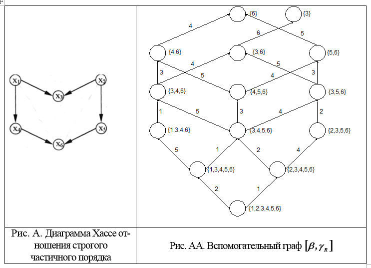
2. For each one-element subset of the set γR, write out its unique numbering. To obtain all the numberings of the subset X, it is necessary to enumerate all adjacent subsets and for each such subset to continue all its numberings. As a result, all numberings of the set Ω will be obtained, i.e. all linear extensions of order R.

The problem is to find all linear additional orderings of a partial order, the diagram of which is shown in Fig. A. There is no information in this regard, for example, whether the alternative dominates

x_{1}

$x_1$ alternative

х_{2}

$_2$ or vice versa, and also similarly for pairs

(х_{3}, х_{6}); (х_{4}, х_{5})

$(_3, _6);(_4, _5)$ ... This means that A is a partial ordering. There are many (22) options to complete to a linear ordering, which it is desirable to bring to a single one. This is possible with the involvement of additional information about the alternatives obtained from a detailed study of the situation.

1. We construct an auxiliary graph [β, γR], starting with the set

(x_{1}, x_{2}, x_{3}, x_{4}, x_{5}, x_{6})

$(x_1, x_2, x_3,x_4, x_5, x_6)$ and below. The number near the graph arc indicates by deleting which maximum element the subset to which this arrow is directed was obtained (Fig. AA).

2. We form the table. AAA to find all numberings of subsets that are vertices of the graph [β, γR]. The table is filled line by line from top to bottom. Each line is the numbering of the subset recorded in the left column of the table (Table AAA).

3. When composing the numbering of a subset X, consisting of k elements, it is necessary to rewrite all previously written (for the previous subset) numbering of subsets Y є γR (x) and assign a number to the element that complements Y to X.

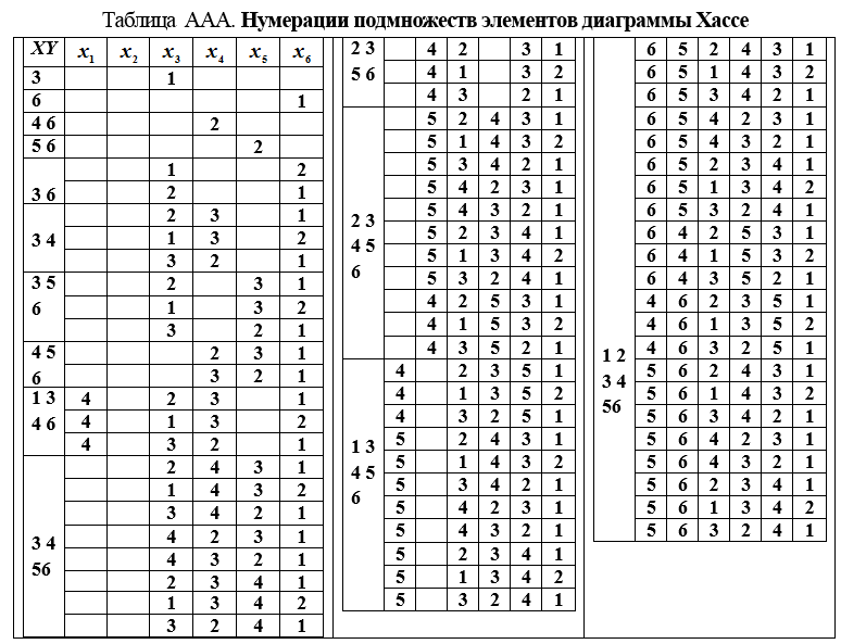
The last (lower) block (Table AAA) contains all the numberings of the linear reordering of the set Ω. A graphical representation of these additional orderings is shown in Fig. AAA.

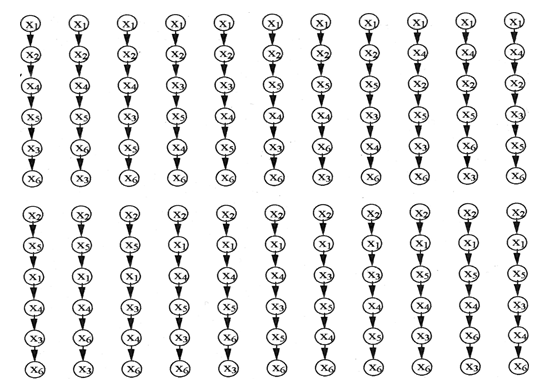
Figure: AAA. Graphical representation of preorders

It should be noted that there are 6 linear orders on a set of 6 elements! or 720, and linear reordering of the set Ω with the relation given by the graph shown in Fig. AA, 22 in total. This is also enough to make a decision.

Are there opportunities to reduce the number of such options? Yes there are.

To reduce the number of linear additional orderings, you need to use additional information.

Additional Information

Let [Ω, R] be the initial relation, then the additional information can be represented as a relation δ on the set Ω, where the condition (x, y) є δ, that is, (x> y) is interpreted as a message that object x dominates object y;

the ratio δ can then be considered as a set of similar messages of information on dominance given as a binary ratio δ, there are two possible cases when using additional information:

the relation graph R∪δ contains contours;
the graph of the relation R∪δ does not contain contours.

In the first case, linear ordering of the set Ω with a given ratio R∪δ on it is performed using the ranking algorithm

considered earlier.

In the second case, the linear ordering of the set Ω with a given ratio R∪δ on it is performed using the linear reordering algorithm

considered above. It should be noted that the relation R∪δ, which does not contain contours, may be nontransitive and, therefore, not a partial order.

For a successful way out of this situation, it is necessary that the additional information δ and the initial ratio R be given in the form of Hasse diagrams, i.e. without explicit indication of transitive links. The value of additional information will be determined by how many times the number of linear additionalorders decreases when it is used.

For example, if information is received that

x_{2}

$x_2$ dominates

x_{4}

$x_4$ , i.e.

x_{2} > x_{4}

$x_2>x_4$ , then the number of linear reorders will decrease from 22 to 19, and if information arrives:

x_{1} > x_{2}

$x_1>x_2$ , then the number of linear preorders is halved. Thus, the question arises: what information will be most valuable, or if you add what ratio δ, the number of additional orderings will decrease the most?

To solve this problem for all pairs of elements

(x_{i}, x_{j})

$(x_i, x_j)$ the sets Ω, which are not included in the relation R, in the lower block of Table. AAA, you need to calculate

n_{i j}

$n_{ij}$ - how many times the item number

x_{i}

$x_i$ more item number

x_{j}

$x_j$ , i.e. element

x_{i}

$x_i$ stands above the element

x_{j}

$x_j$ and

n_{j i}

$n_{ji}$ - how many times an item

x_{j}

$x_j$ stands above the element

x_{i}

$x_i$ ...

The value of additional information about the relationship in this pair will be the higher, the smaller the difference

| n_{i j} - n_{j i} |

$|n_{ij} - n_{ji}|$ ... Greater of numbers

n_{i j}, n_{j i}

$n_{ij}, n_{ji}$ will be equal to the number of reorders of the set [Ω, R∩δ]. For the considered example, we obtain a summary of the characteristics of the graphical representation of the reorders

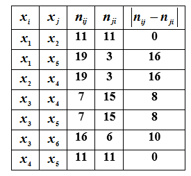
From the analysis of the table it follows that the most useful

information will be information about the relationship in pairs

(x_{1}, x_{2})

$(x_1, x_2)$ and

(x_{4}, x_{5})

$(x_4, x_5)$ ... Obtaining additional information about the relation in any of these pairs leads to a halving of the number of linear additional orderings.

Conclusion

The formulation and solution of the DP is possible only in a situation of many alternatives and the choice of the best one. If there is no choice, then follow the path you are on.

Decisions made by a decision maker are based on his preference, which is described by a preference relation. The presence of the relationship allows you to build a mathematical model for research. Uncertainty in preferences is eliminated by using additional information that is not expert.

Attention is paid to the consideration of measurements and estimates of the values of indicators of properties of objects. Examples of various scales that are often ignored are given.

Possible formulations of ZPR and the information necessary for their solution are listed.

Using a specific numerical example, the application of algebraic methods for solving ZPR is shown, without the use of statistical samples and empirical processing methods.

The method is based on the result of the theorem on the possibility of extending a partial order to a linear (perfect) one.

List of used literature

1. Berge K. Graph theory and its application. - M .: IL, 1962 .-- 320 p.

2. Vaulin AE Discrete mathematics in computer security problems. Part I. SPb .: VKA named after A.F. Mozhaisky, 2015 .-- 219 p.

3. Vaulin AE Discrete mathematics in computer security problems. Ch. II. SPb .: VKA named after A.F. Mozhaisky, 2017 .-- 151 p.

4. Vaulin AE Methods of research of information computing complexes. Issue 2. - L .: VIKI them. A.F. Mozhaisky, 1984 .-- 129 p.

5. Vaulin AE Methodology and methods of analysis of information computing systems. Issue 1.– L .: VIKI im. A.F. Mozhaisky, 1981 .-- 117 p.

6. Vaulin AE Methods of digital data processing: discrete orthogonal transformations. - SPb .: VIKKI them. A.F. Mozhaisky, 1993 .-- 106 p.

7. Kuzmin VB Construction of group solutions in spaces of clear and fuzzy binary relations. - M .: Nauka, 1982. - 168 p.

8. Makarov IM et al. The theory of choice and decision making. - Moscow: Fizmatlit, 1982. –328 p. 52.

9. Rosen V.V. Purpose - optimality - solution. - M .: Radio and communication, 1982. – 169 p.

10. Szpilraijn E Sur Textension de l'ordre partiel. - Fundam. math., 1930, vol. 16, pp. 386-389.

Making decisions. Example