
Today we will tell you how we developed a search system for candidate wells for hydraulic fracturing (HF) using machine learning (hereinafter - ML) and what came of it. Let's figure out why hydraulic fracturing is needed, what ML has to do with it, and why our experience may be useful not only for oilmen.
Under the cut, a detailed statement of the problem, a description of our IT solutions, the choice of metrics, the creation of an ML pipeline, the development of an architecture for the release of a model in prod.
We wrote about why fracturing is done in our previous articles here and here .
Why is machine learning here? On the one hand, hydraulic fracturing is cheaper than drilling, but it is still costly, and on the other hand, it will not be possible to do it at every well - there will be no effect. An expert geologist is looking for suitable places. Since the number of operating companies is large (tens of thousands), options are often overlooked, and the company does not receive possible profits. The use of machine learning can significantly speed up the analysis of information. However, creating an ML model is only half the battle. It is necessary to make it work in a constant mode, connect it to the data service, draw a beautiful interface and make it so that it is convenient for the user to enter the application and solve his problem in two clicks.
Abstracting from the oil industry, one can see that similar tasks are being solved in all companies. Everyone wants to:
A. Automate the processing and analysis of large data streams.
B. Reduce costs and not miss out on benefits.
C. Make such a system fast and efficient.
From the article you will learn how we implemented such a system, what tools we used, and also what bumps we got on the thorny path of introducing ML into production. We are sure that our experience can be of interest to everyone who wants to automate a routine - regardless of the field of activity.
How wells are selected for hydraulic fracturing in the "traditional" way
When selecting candidate wells for hydraulic fracturing, the oilman relies on his extensive experience and looks at different graphs and tables, after which he predicts where to perform hydraulic fracturing. However, no one knows for sure what is going on at a depth of several thousand meters, because it is not so easy to look underground (you can read more in the previous article ). Data analysis by "traditional" methods requires significant labor costs, but, unfortunately, it does not guarantee an accurate forecast of hydraulic fracturing results (spoiler - with ML too).
If we describe the current process of identifying candidate wells for hydraulic fracturing, then it will consist of the following stages: unloading well data from corporate information systems, processing the obtained data, conducting expert analysis, agreeing on a solution, conducting hydraulic fracturing, and analyzing the results. Looks simple, but not quite.
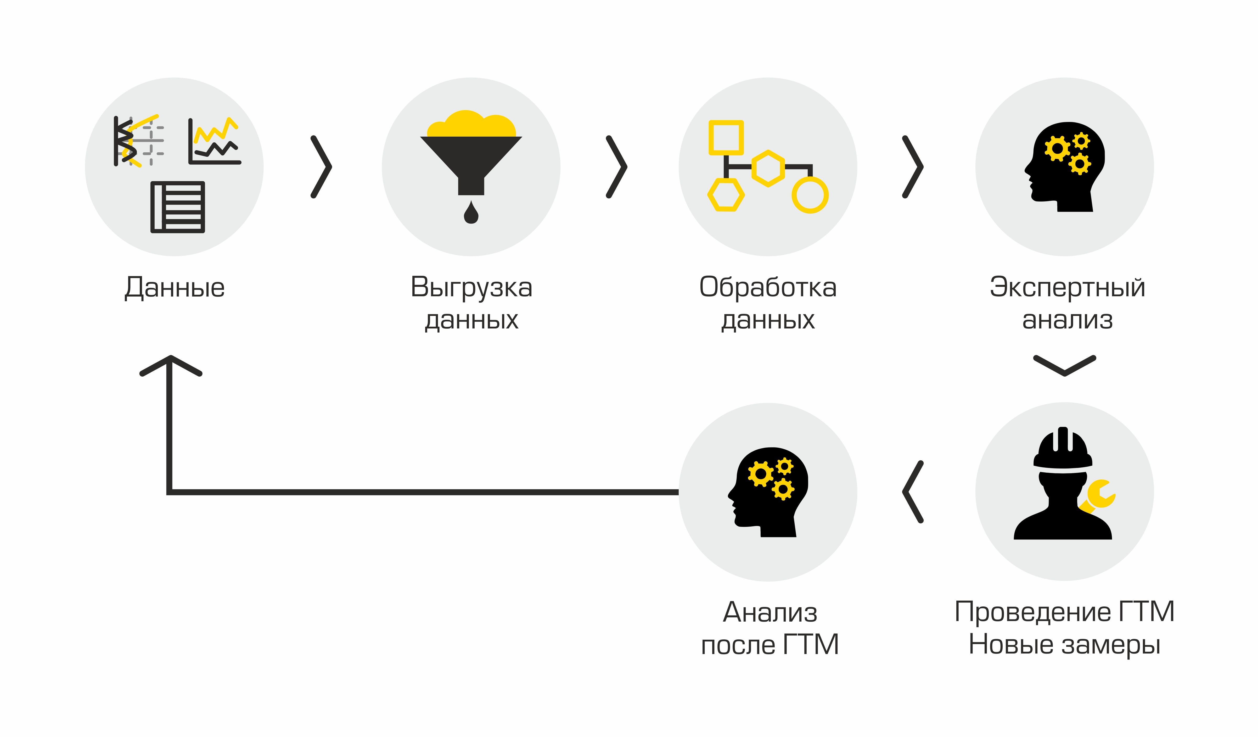
Current selection process for candidate wells
The main disadvantage of this “manual” approach is a lot of routine, volumes grow, people start to drown in work, there is no transparency in the process and methods.
Formulation of the problem
In 2019, our data analysis team faced the task of creating an automated system for the selection of candidate wells for hydraulic fracturing. For us, it sounded like this - to simulate the state of all wells, assuming that right now it is necessary to perform hydraulic fracturing on them, and then rank the wells by the largest increase in oil production and select Top-N wells to which the fleet will travel and take measures to increase oil recovery.
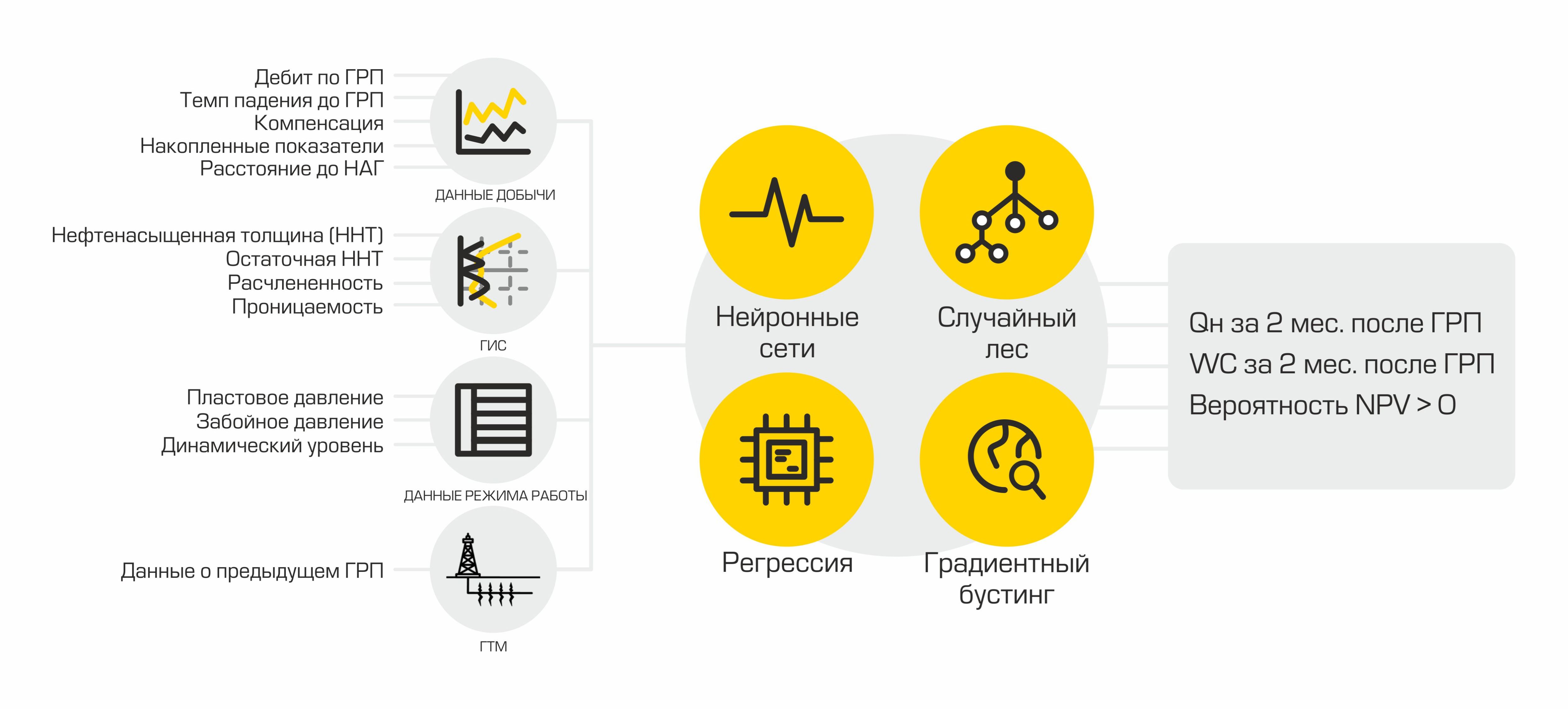
Using ML models, indicators are formed that indicate the feasibility of hydraulic fracturing at a specific well: oil production after the planned hydraulic fracturing and the success of this event.
In our case, the oil production rate is the amount of oil produced in cubic meters per month. This indicator is calculated on the basis of two values: liquid flow rate and water cut. Oilmen call a liquid a mixture of oil and water - it is this mixture that is the product of wells. And the water cut is the proportion of water content in a given mixture. In order to calculate the expected oil production rate after fracturing, two regression models are used: one predicts the fluid flow rate after fracturing, the other predicts water cut. Using the values returned by the model data, oil production forecasts are calculated using the formula:

Fracturing success is a binary target variable. It is determined using the actual value of the increase in oil production, which was obtained after hydraulic fracturing. If the growth is greater than a certain threshold determined by an expert in the domain area, then the value of the success attribute is equal to one, otherwise it is equal to zero. Thus, we form the markup for solving the classification problem.
As for the metric ... The metric should come from the business and reflect the interests of the customer, any machine learning courses tell us. In our opinion, this is where the main success or failure of a machine learning project lies. A group of data scientists can improve the quality of the model for as long as they want, but if it does not increase the business value for the customer in any way, such a model is doomed. After all, it was important for the customer to get an exact candidate with “physical” predictions of the well performance parameters after hydraulic fracturing.
For the regression problem, the following metrics were chosen:

Why is there not one metric, you ask - each reflects its own truth. For fields where average production rates are high, MAE will be large and MAPE will be small. If we take a field with low average production rates, the picture will be the opposite.
The following metrics were chosen for the classification problem:

( wiki ),
Area under the ROC – AUC curve ( wiki ).
Errors we encountered
Error # 1 - to build one universal model for all fields.
After analyzing the datasets, it became clear that the data changes from one field to another. This is not surprising, since deposits, as a rule, have a different geological structure.
Our assumption that if we take and drive all the available data for training into a model, then it will itself reveal the regularities of the geological structure, has failed. The model trained on the data of a particular field showed a higher quality of predictions than the model, which was created using information about all the available fields.
For each field, different machine learning algorithms were tested and, based on the results of cross-validation, one with the lowest MAPE was selected.
Mistake # 2 - Lack of deep understanding of the data.
If you want to make a good machine learning model for a real physical process, understand how this process happens.
Initially, there was no domain expert in our team, and we moved chaotically. Alas, we did not notice the errors of the model when analyzing forecasts, they drew incorrect conclusions based on the results.
Mistake # 3 - lack of infrastructure.
At first, we downloaded many different csv files for different fields and different parameters. At some point, an unbearably large number of files and models have accumulated. It became impossible to reproduce the experiments already carried out, files were lost, and confusion arose.
1. TECHNICAL PART
Today our system of auto-selection of candidates looks like this:
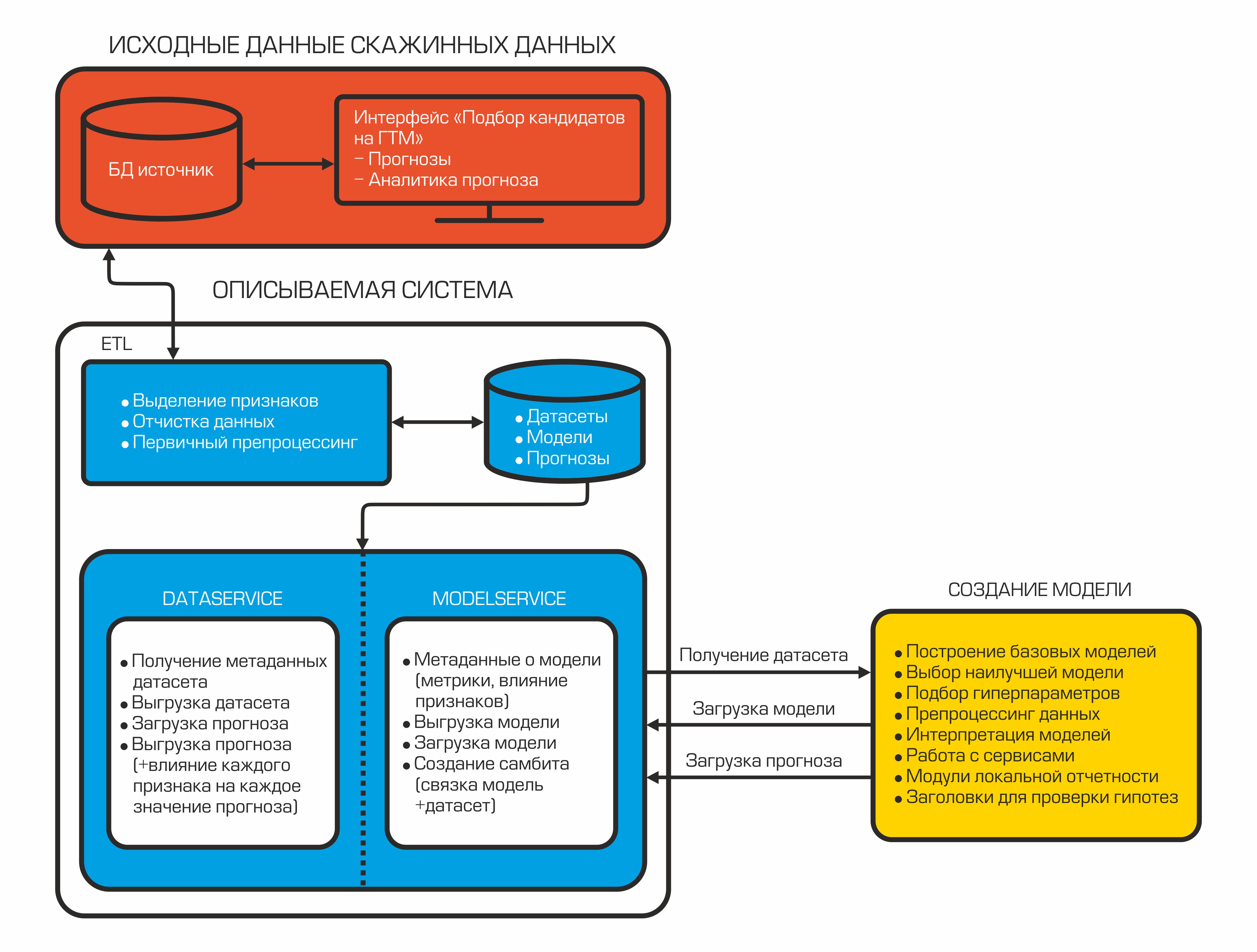
Each component is an isolated container that performs a specific function.
2.1 ETL = Data Load
It all starts with data. Especially if we want to build a machine learning model. We have chosen Pentaho Data Integration as the integration system.

Screenshot of one of the transformations
Main advantages:
- free system;
- a large selection of components for connecting to various data sources and transforming the data stream;
- availability of a web interface;
- the ability to manage via REST API;
- logging.
In addition to all of the above, we had extensive experience in developing integrations for this product. Why is data integration needed in ML projects? In the process of preparing datasets, it is constantly required to implement complex calculations, to bring the data to a single form, to calculate new indicators “along the way”, changes in parameters over time, etc.
For each fact of hydraulic fracturing, more than 400 parameters are unloaded that describe the operation of the well at the time of carrying out activities, operation of adjacent wells, as well as information on previously performed hydraulic fracturing. Further, data transformation and preprocessing takes place.
We chose PostgreSQL as the repository for the processed data. It has a large set of methods for working with json. Since we store the final datasets in this format, this became a decisive factor.
A machine learning project is associated with a constant change in the input data due to the addition of new features, so the Data Vault is used as the database schema (link to the wiki). This storage design scheme allows you to quickly add new data about an object and not violate the integrity of tables and queries.
2.2 Data and Model Services
After combing and calculating the necessary indicators, the data is uploaded to the database. They are stored here and are waiting for the datasinter to take them to create the ML model. For this, there is DataService - a service written in Python and using the gRPC protocol. It allows you to get datasets and their metadata (types of features, their description, dataset size, etc.), load and unload forecasts, manage filtering and division parameters by train / test. Forecasts in the database are stored in json format, which allows you to quickly receive data and store not only the forecast value, but also the influence of each feature on this particular forecast.
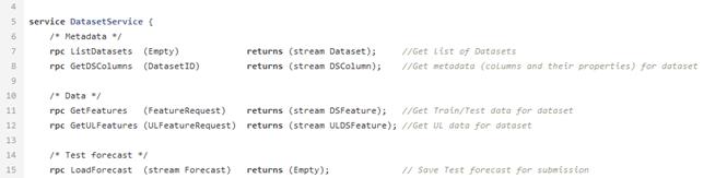
Sample proto file for data service.
When the model is created, it should be saved - for this purpose, the ModelService is used, also written in Python with gRPC. The capabilities of this service are not limited to saving and loading a model. In addition, it allows you to monitor metrics, the importance of features, and also implements a model + dataset connection for the subsequent automatic creation of a forecast when new data appears.
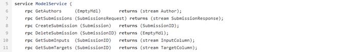
This is how the structure of our model service looks like.
2.3 ML model
At a certain point, our team realized that automation should also affect the creation of ML models. This need was driven by the need to speed up the process of making forecasts and testing hypotheses. And we made the decision to develop and implement our own AutoML library into our pipeline.
Initially, the possibility of using ready-made AutoML libraries was considered, but the existing solutions turned out to be not flexible enough for our task and did not have all the necessary functionality at once (at the request of workers, we can write a separate article about our AutoML). We only note that the framework we have developed contains classes used for preprocessing a dataset, generating and selecting features. As machine learning models, we use a familiar set of algorithms that we have most successfully used before: implementations of gradient boosting from the xgboost libraries, catboost, a random forest from Sklearn, a fully connected neural network on Pytorch, etc. After training, AutoML returns a sklearn pipeline that includes the mentioned classes, as well as the ML model,which showed the best result in cross-validation for the selected metric.
In addition to the model, a report is formed on the influence of any signs on a specific forecast. Such a report allows geologists to look under the hood of a mysterious black box. Thus, AutoML receives the tagged dataset using the DataService and, after training, forms the final model. Next, we can get the final estimate of the quality of the model by loading the test dataset, generating forecasts and calculating quality metrics. The final stage is uploading a binary file of the generated model, its description, metrics to the ModelService, while the forecasts and information about the influence of features are returned to the DataService.
So, our model is placed in a test tube and is ready to be launched into prod. At any time, we can use it to generate forecasts based on new, relevant data.
2.4 Interface
The end user of our product is a geologist, and he needs to somehow interact with the ML model. The most convenient way for him is a module in specialized software. We have implemented it.
The frontend, available to our user, looks like an online store: you can select the desired field and get a list of the most likely successful wells. In the well card, the user sees the predicted growth after hydraulic fracturing and decides for himself whether he wants to add it to the "basket" and consider in more detail.

Module interface in the application.

This is how the well card looks in the appendix.
In addition to the predicted oil and liquid gains, the user can also find out which features influenced the proposed result. The importance of features is calculated at the stage of creating a model using the shap method , and then loaded into the software interface with DataService.
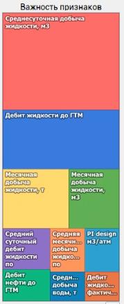
The application clearly shows which features were the most important for model predictions.
The user can also look at analogs of the well of interest. The search for analogs is implemented on the client side using the Kd tree algorithm .
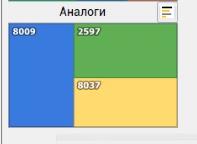
The module displays wells with similar geological parameters.
2. HOW WE IMPROVED THE ML MODEL

It would seem that it is worth running AutoML on the available data, and we will be happy. But it so happens that the quality of the forecasts obtained automatically cannot be compared with the results of datasinters. The fact is that analysts often put forward and test various hypotheses to improve models. If the idea improves the accuracy of forecasting on real data, it is implemented in AutoML. Thus, by adding new features, we have improved automatic forecasting enough to move on to creating models and forecasts with minimal involvement of analysts. Here are some hypotheses that have been tested and implemented in our AutoML:
1. Changing the filling method
In the very first models, we filled in almost all the gaps in the characteristics with the mean, except for the categorical ones - for them the most common meaning was used. Later, with the joint work of analysts and an expert, in the domain area, it was possible to select the most suitable values to fill in the gaps in 80% of features. We also tried a few more fill-in methods using the sklearn and missingpy libraries. The best results were obtained with constant filling and KNNImputer - up to 5% MAPE.

Results of an experiment on filling the gaps with different methods.
2. Generation of features
Adding new features is an iterative process for us. To improve the models, we try to add new features based on the recommendations of a domain expert, based on experience from scientific articles and our own conclusions from the data.

Testing the hypotheses put forward by the team helps to introduce new features.
One of the first were the features identified on the basis of clustering. In fact, we simply selected clusters in the dataset based on geological parameters and generated basic statistics for other characteristics based on clusters - this gave a small increase in quality.
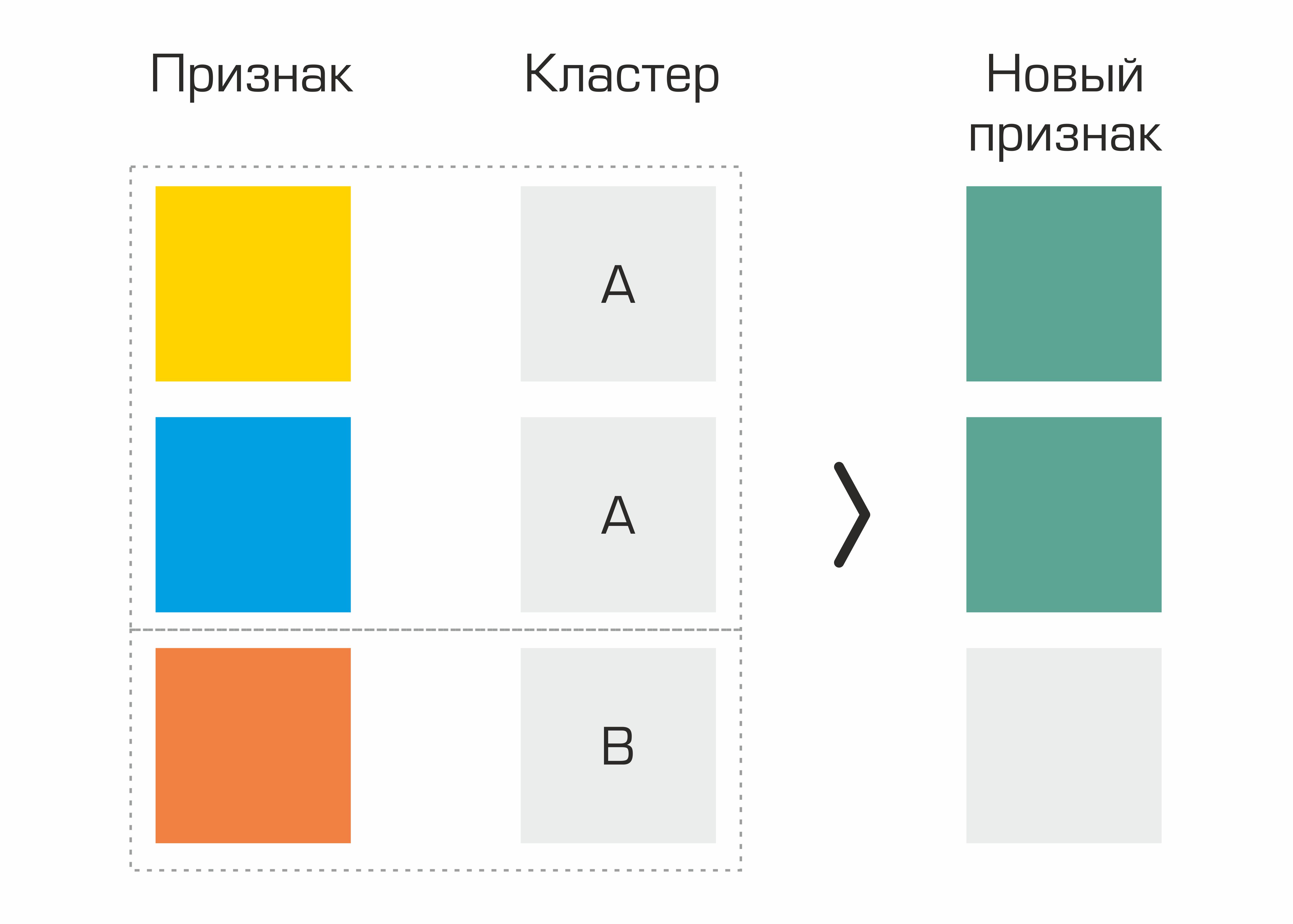
The process of creating a feature based on the selection of clusters.
We also added the signs that we invented when immersed in the domain region: cumulative oil production normalized to the age of the well in months, cumulative injection normalized to the age of the well in months, parameters included in the Dupuis formula. But the generation of the standard set from PolynomialFeatures from sklearn did not give us an increase in quality.
3.
Feature selection We performed feature selection multiple times: both manually together with a domain expert and using standard feature selection methods. After several iterations, we decided to remove from the data some features that do not affect the target. Thus, we managed to reduce the size of the dataset, while maintaining the same quality, which made it possible to significantly speed up the creation of models.
And now about the received metrics ...
At one of the fields, we obtained the following model quality indicators:

It should be noted that the result of hydraulic fracturing also depends on a number of external factors that are not predicted. Therefore, we cannot talk about reducing MAPE to 0.
Conclusion The
selection of candidate wells for hydraulic fracturing using ML is an ambitious project that brought together 7 people: data engineers, datasunters, domain experts and managers. Today, the project is actually ready for launch and is already being tested at several subsidiaries of the Company.
The company is open to experimentation, so about 20 wells were selected from the list and fractured. The deviation of the forecast with the actual value of the starting oil production rate (MAPE) was about 10%. And this is a very good result!
Let's not be cunning: especially at the initial stage, several of our proposed wells turned out to be unsuitable options.
Write questions and comments - we will try to answer them.
Subscribe to our blog, we have many more interesting ideas and projects, which we will definitely write about!