👨🏽‍🎤 🙈 ✉️ Options: put-call hover, Brownian move. Educational program for a geek, part 7 🎼 💛 👌🏾

This is the second part of the story about options, where we will deal with put-call soaring, the condition of no market arbitrage, get acquainted with the ideas of hedging and replication, and talk about what Brownian motion is and how it is related to modeling the behavior of the rate of a financial asset over time.

There will be some math to get a better understanding of the details

This post is a transcript of my video lectures " Put-call hover and the condition for the absence of arbitrage ", " Brownian motion ", created as part of the Finmath for Fintech course.

Put-call hover. An example of using the no arbitrage condition to analyze the price of a portfolio of instruments

So, from the previous part, we know what the payouts for a put and call option look like on expiry (the point in time when the right provided by the option can be exercised), but we would also like to know how to calculate the option for other periods of time. To do this, we need to build a mathematical model using a more complex mathematical apparatus. However, before we do that, let's look at the put-to-call parity relationship, which is not complicated and very useful in practice.

Recall that a European option is a contract under which the buyer of the contract receives the right, but not the obligation, to buy or sell some underlying asset at a predetermined price at a certain moment in the future in the contract.

The underlying asset can be a stock or a currency rate. The market rate for the underlying asset is called the spot, and in the formulas, the value of the spot at the time

t

$t$ denoted as

S_{t}

$S_t$ ...

An option that gives the right to buy the underlying asset is called a call option. The right to sell is a put option. The price at which the option gives the right to conclude a deal in the future is called a strike, denoted

K

$K$ ...

The pre-agreed time in the contract at which the option can be used is the expiry time of the option (expiry) -

T

$T$ ... The value of the underlying asset rate at the time of expiry is indicated by

S_{T}

$S_T$ ...

Let's build payment schedules for expiry. We have a certain underlying asset - its expiry price:

S_{T}

$S_T$ as well as payment

P

$P$ we receive. Payout schedules will be in these coordinates

S_{T}, P

$S_T, P$ ... Let's set

K

$K$ - strike level on the axis

S_{T}

$S_T$ ...

The first option we'll draw is a call option. We bought a call option.

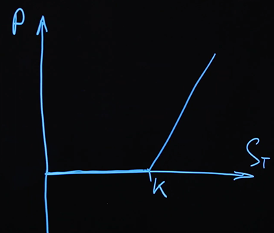
This is also called a “long” call option , a plus sign position on that option. But we can also sell options, this is called short .

The second option we'll draw will be a short put .

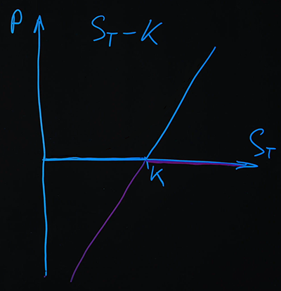
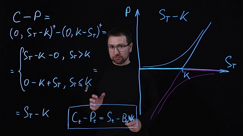
In the graph, we can see that when we added the two payments, we got a simple linear function, which is defined as (

S_{T} - K

$S_T-K$ ). The same result can be obtained analytically. We have a call option position with a plus sign and a put option with a minus sign:

C - P

$C-P$

Let's use the analytical formulas that we already know:

m a x (0, S_{T} - K) - m a x (0, K - S_{T})

$max(0, S_T-K)-max(0, K-S_T)$ ...

To expand the brackets, we have to consider two separate cases where

S_{T} > K

$S_T>K$ and

S_{T} < K

$S_T<K$ ...

We have the following system:

{\begin{cases} S_{T} - K - 0, S_{T} > K \\ 0 - K + S_{T}, S_{T} \leq K \end{cases}

$\begin{cases} S_T-K-0, S_T>K \\ 0-K+S_T, S_T≤K \end{cases}$

In both cases, you get the same simple formula:

S_{T} - K

$S_T-K$ ...

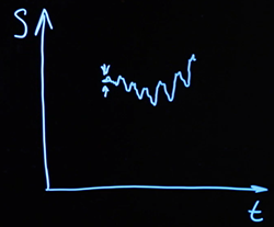
Thus, payments are in any case described by the same formula, regardless of the price of the underlying asset realized at the time of expiry. Again, I remind you that the payments that we have drawn are payments (and hence the cost) of the options at the time of expiry. In the case of option prices at some other point in time, they are described by some other, more complex functions. I will draw them conditionally for now.

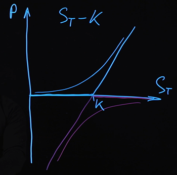
We know that for this combination at the time of expiry, the payout is determined by the formula

S_{T} - K

$S_T-K$ , for any value

S_{T}

$S_T$ ... If we find some other combination of instruments that will give the same payout at the time of expiry, then we can say that the cost of such a combination of instruments and combination

C - P

$C-P$ should be the same.

If this were not the case, then today you can buy the cheaper of these combinations of instruments and sell the more expensive one, thereby making a profit. And since these two combinations give the same payout on expiry, and we took them with opposite signs, the total payout is guaranteed to be zero. Such a transaction, which gives a guaranteed income without risk, simply due to the imbalance in the prices of instruments in the market, is called arbitrage.... Mathematical theories for calculating the prices of instruments usually include the assumption that the market is free of arbitrage. This assumption matches reality well enough. Arbitration opportunities in the market, if they do arise, do not last long. Finding and using them is not easy. So normally this assumption works well.

From the condition that the market is free from arbitrage, it follows that the combination

C - P

$C-P$ will be at any time

t \leq T

$t≤T$ (not only

T

$T$ ) cost the same as any combination of instruments, the payout of which at the moment of time

T

$T$ will be equal

S_{T} - K

$S_T-K$ ... This combination is easy to make by purchasing the underlying asset

S

$S$ and borrowing money in such an amount that at the time of expiry it will be necessary to return an amount equal to

K

$K$ ... When dealing with financial instruments, such debt is equivalent to selling a zero-coupon bond (bond), which pays

K

$K$ at the moment

T

$T$ ... You can read more about bonds and interest in the previous posts in this series ( Value of money, types of interest, discounting and forward rates. Educational program for a geek, part 1 and Bonds: coupon and zero-coupon, yield calculation. Educational program for a geek, part 2 ) ...

So, a portfolio from a call option and a portfolio from a put option is equal to the combination of a long on the underlying asset and a short bond, which would give one payout per expiry with a par

K

$K$ ...

C_{t} - P_{t} = S_{t} - B_{T} K

$C_t-P_t=S_t-B_TK$

This ratio is independent of the model that we could build for the underlying asset rate. It does not even depend on how we consider discounting, and this follows from the absence of arbitrage in the market. We have compiled one portfolio, considered all possible options, how much it can cost on expiry, found out that in all future options it costs exactly the same. Therefore, if another portfolio has exactly the same expiry payout, then their price should be the same.

So, we got the ratio for a portfolio of call and put options. We compiled a portfolio, examined what kind of payment it will have at the time of expiry, found out that the payment is described by one linear equation. Unlike the payout function for call and put options, each of which has two sections, more and less

S_{T}

$S_T$ ... This allows you to build a portfolio of simpler instruments that will give the same payout on expiry in any situation. The price of these two portfolios will be equal at any moment of time, not just at the moment of expiry. This is guaranteed by the condition that there is no arbitrage in the market. If there is arbitrage on the market and this equality is not satisfied, then we, accordingly, can buy one of these portfolios, sell another and get a guaranteed win. This ratio does not depend on any mathematical models that we could build, for example, for the price of the underlying asset. This ratio must be fulfilled in any model.

You can also look at this ratio like this. We have compiled a portfolio of several assets with the same risk. The formula can be rewritten to collect assets that carry the risk associated with the underlying asset on the one hand. That is, we can eliminate all the risk inherent in these instruments, i.e. uncertainty associated with the future price of the underlying asset, knowing exactly how much such a package is worth.

C_{t} - P_{t} - S_{t} = - B_{t} K

$C_t-P_t-S_t=-B_tK$

This way of getting rid of risk is called hedging . We compose a portfolio of several instruments in which some of the same risk is embedded, but we select them in such proportions that these risks mutually balance each other and we get rid of it. This idea is used in other, more complex hedging strategies. The case under consideration is very simple, it allows you to work only with a certain combination of options.

If we look at this idea from the other side, then we could express one of these tools through others. For example, if we have one thing in the market, a put option, then we will automatically receive a call option as well. In this case, it will be replication- we replicated the payment of one product through others. Hedging and replication are closely related to each other, mathematically, they are very similar calculations.

In this case, we have a very simple situation, and in order to completely hedge the risk or replicate the payout, we just need to make a portfolio once, and then we wait until the moment of expiry, the payout is already guaranteed to us. This is called static replication ( static hedging). This is a rare case and usually does not work. In order to achieve this effect more generally, it will be necessary to resort to dynamic hedging strategies. That is, we will make a portfolio once, but then we will constantly need to add something to it or change something there, so that the payment at the time of expiry turns out exactly as we want.

Here's an interesting ratio of put-call soaring. Despite the fact that the math is very simple, in his example you can see several very important ideas that are applied in a more complex case - the application of the no-arbitrage condition, replication of payments and hedging of risks. This is where we finish with this simple relationship and can move on to building a more complex model.

We would like to build a model that would give not only the ratio between call and put options, but also the option price as a function of the values observed in the market. This will require a more complex mathematical theory.

What is Brownian motion and who is Robert Brown. How to simulate Brownian motion on a computer. What is geometric Brownian motion

What we have considered so far allowed us to get by with a very simple mathematical apparatus, in fact, school mathematics. To move on and build a more complex mathematical model, this will not be enough for us, and elements of "adult" mathematics are required. Therefore, the general approach to further presentation will look like this: I will give illustrative examples from which it will be clear how the mathematical apparatus works in a simple case, and I will also give formulations and theorems that we will use. I will not prove these theorems. Those who are interested in the math part can refer to the corresponding textbooks and video courses.

The first concept we need is Brownian motion... Let's remember what this term means in physics. This will be a kind of clear example of how this process will be arranged in our formal mathematical model.

I think that many have the term " Brownian motion"associated with the school physics curriculum. Many believe that the person who introduced this concept into scientific circulation was a physicist by the name of Brown and, judging by his last name, was an Englishman. Interestingly, all of these assumptions are wrong. First, the name of this scientist was Robert Brown, which in Russian should be read as “Robert Brown”. Although this might not be obvious for an educated person of the 18th – 19th centuries, whose first foreign language was French and the second German. Secondly, he was not an Englishman - he was a Scotsman, which, as we understand, is not at all the same thing. But the most interesting thing is that he was not a physicist - he was a botanist. When he conducted and described his famous experiment, he was studying pollen particles under a microscope. The specimen on the slide was prepared in the form of a drop of liquid, in which pollen particles were placed in order toso that the pollen does not fly away from every draft and it can be viewed calmly.

Brown's attention was drawn to the fact that what he sees in the microscope eyepiece is not a static picture. He observed, relatively speaking, a round particle that made a chaotic motion. Today we know that this phenomenon has a simple explanation. There are many molecules in the solution around this particle, which very often interact with it in a random direction, as a result of which the particle makes some kind of complex motion.

If we depict its movement, it will be some random trajectory.

What does this have to do with our subject area? In fact, the analogy is straightforward. We consider the rate of a financial asset over time. A lot of random factors act on it, as well as on that particle, at each moment of time. We do not see them, just as Robert Brown did not see individual molecules through a microscope.

The cumulative effect of these random factors leads to a change in the course of the asset - just as the cumulative effect of molecules leads to the displacement of a pollen particle. These processes occur continuously in time. And thus the rate of the financial asset is realized. The dependence of the course on time is obtained randomly, and therefore such a trajectory is called Brownian motion. In our case, this is a one-dimensional Brownian motion, since random deviations occur only about one axis.

The formal mathematical model of the process that we will use is associated with the name of another scientist, the American mathematician Norbert Wiener. It looks like this. We are considering a continuous time function. Because the

t

$t$ is continuous, then the function

W (t)

$W(t)$ continuous.

It contains a random component, which is mathematically determined as follows:

△ W_{△ t}

$\triangle W_{\triangle t}$ - independent provided that the time increments do not intersect.

Function increment from time point

t

$t$ until the moment

t + s

$t+s$ normally distributed with parameters 0 and

s

$s$ (the length of the time interval).

W_{t + s} - W_{t} \sim N (0, s)

$W_{t+s}-W_t∼N(0,s)$

In what follows, we will see that it is very important to be able to generate such paths on a computer - this is necessary for many computational methods. How could we do this? Time, which is continuous in a theoretical mathematical model, we divide on a computer into some increments, usually with a fixed step. We create a certain starting point from which our process starts, with coordinates

W_{0}; t_{0}

$W_0;t_0$ ... Then, for each subsequent time step, we generate a random variable with such a distribution, and move it one step. We do this at every point. The result is a broken line.

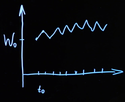
Somewhere the increment turned out with a plus sign, somewhere with a minus sign. As a result, at each specific point, the value of the entire process is determined by the cumulative sum of all these random variables. In order to be able to scale the average displacement per unit of time, we can also introduce an additional parameter, usually denoted by the letter

σ

$\sigma$ (as for the normal distribution). We can consider the function

σ W_{t}

$\sigma W_t$ where

W_{t}

$W_t$ Is the standard Brownian motion, and

W_{t}

$W_t$ has a wider or narrower variance, depending on what we need.

With such a process in place, we would like to build a mathematical model that would help us calculate the price of options. Let us construct equations according to the same principle as we did with interest for discounting in continuous time. This will be some kind of differential equation.

If we were solving the problem of calculating interest on a certain amount

P

$P$ in continuous time, then for a small time step we would have the correct relation

△ P = r P △ t

$\triangle P=rP\triangle t$ or

\frac{△ P}{P} = r △ t

$\frac{\triangle P}{P}=r\triangle t$ ,

where

r

$r$ Is a risk-neutral interest rate. And going to the limit

Δ t \to d_{t}

$Δt →d_t$ , we obtain the differential equation

\frac{d P}{P} = r d t

$\frac{dP}{P}=rdt$ ...

From it we get the already familiar formula for discounting in continuous time

P = P_{0} e^{r t}

$P=P_0e^{rt}$ where

P_{0}

$P_0$ Is the initial value.

I would like to adapt this logic of reasoning for a mathematical model of an asset, the price of which in the future depends on random factors. The relative change in the price of our asset is characterized by a certain parameter, an analogue of the risk-neutral rate (in this case, the parameter characterizes our underlying asset, it is not a risk-neutral rate). Let us add to this expression a probabilistic component that would be described by Brownian motion.

\frac{Δ S}{S} = μ Δ t + σ Δ W

$\frac{ΔS}{S}=μΔt+σΔW$

We practically have a result. Let's move to the limit and get an equation very similar to the one we easily solved for continuous time discounting.

\frac{d S}{S} = μ d t + σ d W

$\frac{dS}{S}=μdt+σdW$

But there is a technical problem. The point is that Brownian motion (Wiener process), as we defined it, is a continuous function of time, but it is not differentiable in the sense of classical mathematical analysis. This can be formally proved (we omit the proof).

In order to construct such a model mathematically rigorously, it is necessary to determine what meaning we put into the expression

d W

$dW$ ... For this, it is necessary to use a stochastic differential, the name of which is associated with the name of another mathematician - the Ito differential . It obeys different rules than those we are used to in conventional calculus.

For reference, I will write the results that we need regarding this mathematical apparatus. The Ito differential obeys such rules.

If

d x = a (x, t) d t + b (x, t) d W_{t}

$dx=a(x,t)dt+b(x,t)dW_t$ ,

then for

f (x, t)

$f(x,t)$ :

d f = \frac{\partial f}{\partial t} d t + \frac{\partial f}{\partial x} d x + \frac{1}{2} \frac{\partial^{2} f}{\partial x^{2}} d x^{2}

$df=\frac{∂f}{∂t}dt+\frac{∂f}{∂x}dx+\frac{1}{2}\frac{∂^2f}{∂x^2}dx^2$ ...

This rule differs from the way we differentiate a function of two variables in conventional calculus. If we have two independent variables, in ordinary calculus we take partial derivatives and stop at the first two terms of the expansion. The third component of the expansion of the differential of a function in the Ito formula appears precisely because we are working not with ordinary functions, but with a random, stochastic process. We take this result ready-made, without proving it.

There is more to be said about

d x^{2}

$dx^2$ in the last equation. By condition

d x = a (x, t) d t + b (x, t) d W_{t}

$dx=a(x,t)dt+b(x,t)dW_t$ , if we square it, then there will be terms with factors

d t d W_{t}

$dt dW_t$ ,

d t^{2}

$dt^2$ ,

d W_{t}^{2}

$dW^2_t$ ... To apply the Ito formula, you need to take:

d t d W_{t} = 0

$dt dW_t=0$ ;

d t^{2} = 0

$dt^2=0$ ;

d W_{t}^{2} = d t

$dW^2_t=dt$ ...

All these rules become natural if you understand what the Ito integral is, but for our purposes now it is enough to know how to correctly apply the Ito formula.

And now we can overcome our technical complexity, since we know how to operate with an object

σ d W

$σdW$ ...

As a variable

x

$x$ we have the underlying asset rate

S

$S$ , we can express it:

d S = S μ d t + σ S d W_{t}

$dS=Sμdt+σSdW_t$ ...

Next, we know how to write the differential of the function, where there is

S

$S$ and

t

$t$ ... Let's see what is the differential of the function

f (S, t) = l n (S)

$f(S, t)=ln⁡(S)$ ...

d l n S = d f = \frac{\partial f}{\partial t} d t + \frac{\partial f}{\partial S} d S + \frac{1}{2} \frac{d^{2} f}{d S^{2}} d S^{2} =

$dln S = df = \frac{∂f}{∂t}dt+\frac{∂f}{∂S}dS+\frac{1}{2}\frac{d^2f}{dS^2}dS^2=$

= 0 d t + \frac{1}{S} (S μ d t + σ S d W_{t}) - \frac{1}{2} \frac{1}{S^{2}} σ^{2} S^{2} d t

$=0 dt+\frac{1}{S}(Sμdt+σSdW_t)-\frac{1}{2}\frac{1}{S^2}\sigma^2 S^2 dt$

Now, collecting the terms, we get an expression for the logarithm

S

$S$ ...

d ㏑ S = (μ - \frac{σ^{2}}{2}) d t + σ d W

$d㏑S=(μ-\frac{\sigma^2}{2})dt+σdW$

Now we know what is equal to

㏑ S

$㏑S$ (note that it has a normal distribution). We are interested directly in the expression for

S

$S$ ...

S = S_{0} e^{μ t} e x p (σ W_{t} - \frac{σ^{2}}{2} t)

$S=S_0 e^{μt}exp(σW_t-\frac{\sigma^2}{2}t)$

The above expression describes geometric Brownian motion . It represents some exponential growth with the parameter

μ

$\mu$ which initially starts at point

S_{0}

$S_0$ , and noise is superimposed around this exponent according to the expression

e x p (σ W_{t} - \frac{σ^{2}}{2} t)

$exp(\sigma W_t-\frac{\sigma^2}{2}t)$ ... This can already be read on a computer, we can generate paths of Brownian motion. We will get some possible realizations of our path for the underlying asset rate. There are two parameters in this equation:

σ

$\sigma$ - variance and

μ

$\mu$ - drift. They correspond to the variance of the normal distribution and the bias of the normal distribution for

㏑ S

$㏑S$ ... As I said, it is now possible to simulate on a computer, but there is one more theoretical component that we need to introduce so that we can calculate the price of the options using this process. Next we will talk about risk-neutral measure.

All articles in this series

Options: put-call hover, Brownian move. Educational program for a geek, part 7

Put-call hover. An example of using the no arbitrage condition to analyze the price of a portfolio of instruments

What is Brownian motion and who is Robert Brown. How to simulate Brownian motion on a computer. What is geometric Brownian motion

More articles: