We continue our research on the situation in the United States with the shooting of police officers and the crime rate among representatives of the white and black (African American) races. Let me remind you that in the first part I talked about the premises of the study, its goals and accepted reservations / assumptions; and the second part was a demonstration of the analysis of the relationship between race, crime and death at the hands of law enforcement agencies.
Let me also remind you of the intermediate conclusions made on the basis of statistical observations (for the period from 2000 to 2018):
In quantitative (absolute) terms, there are more white police victims than blacks.
On average, the police kill 5.9 per million blacks and 2.3 per million whites (2.6 times more blacks).
The annual spread (deviation) in the deaths of blacks at the hands of the police is almost twice as high as in the data for white victims.
Police casualties among whites are monotonously increasing (on average by 0.1 - 0.2 per year), while casualties among blacks have returned to the 2009 level after a peak in 2011 - 2013.
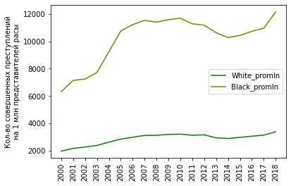
Whites commit twice as many crimes as blacks in absolute terms, but 3 times less in relative terms (per million members of their race).
White crime has been growing relatively monotonously throughout the entire period (it has doubled in 18 years). Black crime is also on the rise, but in leaps and bounds. Over the entire period, crime among blacks also doubled (similar to whites).
Death at the hands of the police is associated with criminality (the number of crimes committed). Moreover, this correlation is heterogeneous across races: for whites it is close to ideal, for blacks it is far from such.
Deaths in meetings with the police are on the rise "in response" to the rise in crime, with a lag of several years (especially seen in the data among blacks).
White criminals are slightly more likely to be killed by the police than black ones.
, , , , , .
, , , , " " (All Offenses) "". , , " " , , , ( ) , . , (, , )... , !
" "
, , ,
df_crimes1 = df_crimes1.loc[df_crimes1['Offense'] == 'All Offenses']:
df_crimes1 = df_crimes1.loc[df_crimes1['Offense'].str.contains('Assault|Murder')], , (Assault) (Murder). , , .
. .
:
, , ( ).
:


:
White_promln_cr | White_promln_uof | Black_promln_cr | Black_promln_uof | |
|---|---|---|---|---|
White_promln_cr | 1.000000 | 0.684757 | 0.986622 | 0.729674 |
White_promln_uof | 0.684757 | 1.000000 | 0.614132 | 0.795486 |
Black_promln_cr | 0.986622 | 0.614132 | 1.000000 | 0.680893 |
Black_promln_uof | 0.729674 | 0.795486 | 0.680893 | 1.000000 |
, (0.68 0.88 0.72 ). , , , .. , .
, "" - :

, . - , .
, .
, - ! :)
, :
, , , : , , . .
51 1991 2018 , :
homicide:
rape legacy: ( - 2013 .)
rape revised: ( - 2013 .)
robbery:
aggravated assault:
property crime:
burglary: /
larceny:
motor vehicle theft:
arson:
(violent crime), .
51 2000 2018 , ( - . ). , 4 (, , ).
:
import pandas as pd, numpy as np

CRIME_STATES_FILE = ROOT_FOLDER + '\\crimes_by_state.csv'
df_crime_states = pd.read_csv(CRIME_STATES_FILE, sep=';', header=0,
                              usecols=['year', 'state_abbr', 'population', 'violent_crime'])
:
year | state_abbr | population | violent_crime | |
|---|---|---|---|---|
0 | 2016 | AL | 4860545 | 25878 |
1 | 1996 | AL | 4273000 | 24159 |
2 | 1997 | AL | 4319000 | 24379 |
3 | 1998 | AL | 4352000 | 22286 |
4 | 1999 | AL | 4369862 | 21421 |
... | ... | ... | ... | ... |
1423 | 2000 | DC | 572059 | 8626 |
1424 | 2001 | DC | 573822 | 9195 |
1425 | 2002 | DC | 569157 | 9322 |
1426 | 2003 | DC | 557620 | 9061 |
1427 | 2016 | DC | 684336 | 8236 |
1428 rows × 4 columns
df_crime_states = df_crime_states.merge(df_state_names, on='state_abbr')
df_crime_states.dropna(inplace=True)
df_crime_states.sort_values(by=['year', 'state_abbr'], inplace=True)
, :
df_crime_states['crime_promln'] = df_crime_states['violent_crime'] * 1e6 / df_crime_states['population'], 2000 2018 , :
df_crime_states_agg = df_crime_states.groupby(['state_name', 'year'])['violent_crime'].sum().unstack(level=1).T
df_crime_states_agg.fillna(0, inplace=True)
df_crime_states_agg = df_crime_states_agg.astype('uint32').loc[2000:2018, :]
19 ( , .. 2000 2018) 51 ( ).
-10 :
df_crime_states_top10 = df_crime_states_agg.describe().T.nlargest(10, 'mean').astype('int32')count | mean | std | min | 25% | 50% | 75% | max | |
|---|---|---|---|---|---|---|---|---|
state_name | ||||||||
California | 19 | 181514 | 19425 | 153763 | 165508 | 178597 | 193022 | 212867 |
Texas | 19 | 117614 | 6522 | 104734 | 113212 | 121091 | 122084 | 126018 |
Florida | 19 | 110104 | 18542 | 81980 | 92809 | 113541 | 127488 | 131878 |
New York | 19 | 81618 | 9548 | 68495 | 75549 | 77563 | 85376 | 105111 |
Illinois | 19 | 62866 | 10445 | 47775 | 54039 | 64185 | 69937 | 81196 |
Michigan | 19 | 49273 | 5029 | 41712 | 44900 | 49737 | 54035 | 56981 |
Pennsylvania | 19 | 46941 | 5066 | 39192 | 41607 | 48188 | 51021 | 55028 |
Tennessee | 19 | 41951 | 2432 | 38063 | 40321 | 41562 | 43358 | 46482 |
Georgia | 19 | 40228 | 3327 | 34355 | 38283 | 39435 | 41495 | 47353 |
North Carolina | 19 | 37936 | 3193 | 32718 | 34706 | 38243 | 40258 | 43125 |
:
df_crime_states_top10 = df_crime_states_agg.loc[:, df_crime_states_agg_top10.index]
plt = df_crime_states_top10.plot.box(figsize=(12, 10))
plt.set_ylabel('-   (2000 - 2018)')
"" . - (, ); :)
, (, , ), (, ).
, . -10 2018 :
df_crime_states_2018 = df_crime_states.loc[df_crime_states['year'] == 2018]
plt = df_crime_states_2018.nlargest(10, 'population').sort_values(by='population').plot.barh(x='state_name', y='population', legend=False, figsize=(10,5))
plt.set_xlabel(' (2018)')
plt.set_ylabel('')
, , . :
#      2000 - 2018  (   )
df_corr = df_crime_states[df_crime_states['year']>=2000].groupby(['state_name']).mean()
#     ""  "- "
df_corr = df_corr.loc[:, ['population', 'violent_crime']]
df_corr.corr(method='pearson').at['population', 'violent_crime']
- 0.98. !
-:
plt = df_crime_states_2018.nlargest(10, 'crime_promln').sort_values(by='crime_promln').plot.barh(x='state_name', y='crime_promln', legend=False, figsize=(10,5))
plt.set_xlabel('-    1 . . (2018)')
plt.set_ylabel('')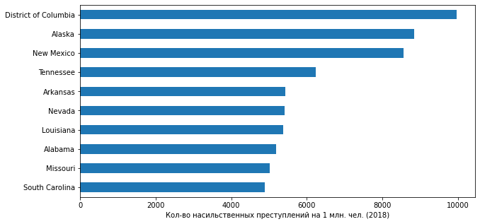
! : (.. ) ( 700+ . 2018 .) (- 2 . .) , , , ...
. folium:
import folium- 2018 . :
FOLIUM_URL = 'https://raw.githubusercontent.com/python-visualization/folium/master/examples/data'
FOLIUM_US_MAP = f'{FOLIUM_URL}/us-states.json'

m = folium.Map(location=[48, -102], zoom_start=3)

folium.Choropleth(
    geo_data=FOLIUM_US_MAP,
    name='choropleth',
    data=df_crime_states_2018,
    columns=['state_abbr', 'violent_crime'],
    key_on='feature.id',
    fill_color='YlOrRd',
    fill_opacity=0.7,
    line_opacity=0.2,
    legend_name='   2018 .',
    bins=df_crime_states_2018['violent_crime'].quantile(list(np.linspace(0.0, 1.0, 5))).to_list(),
    reset=True
).add_to(m)

folium.LayerControl().add_to(m)

m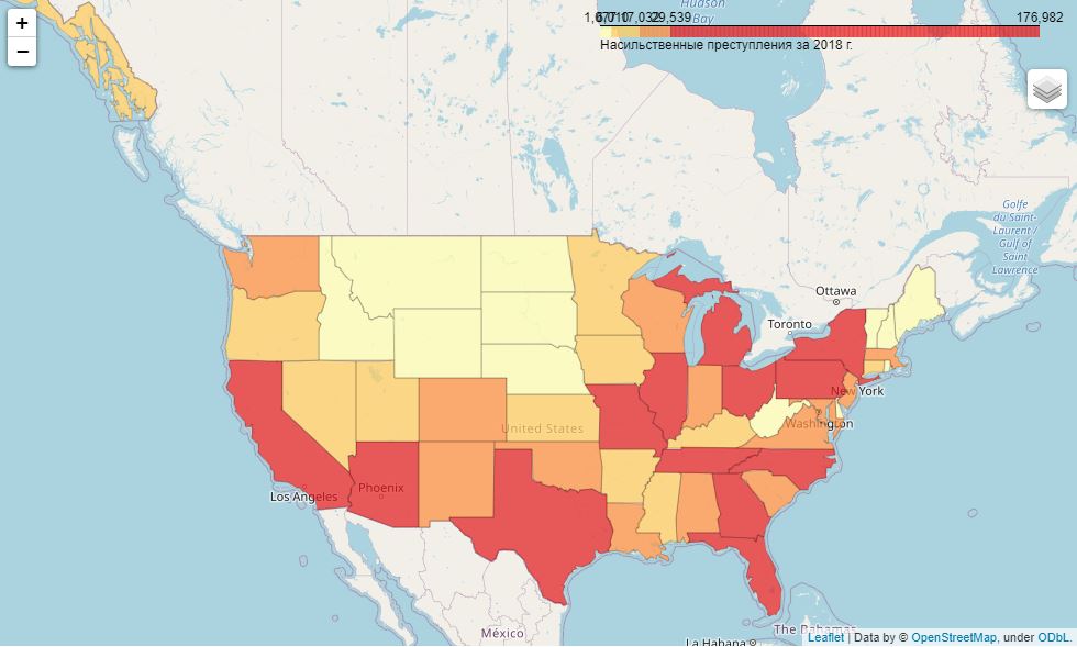
( 1 ):
m = folium.Map(location=[48, -102], zoom_start=3)

folium.Choropleth(
    geo_data=FOLIUM_US_MAP,
    name='choropleth',
    data=df_crime_states_2018,
    columns=['state_abbr', 'crime_promln'],
    key_on='feature.id',
    fill_color='YlOrRd',
    fill_opacity=0.7,
    line_opacity=0.2,
    legend_name='   2018 . ( 1 . )',
    bins=df_crime_states_2018['crime_promln'].quantile(list(np.linspace(0.0, 1.0, 5))).to_list(),
    reset=True
).add_to(m)

folium.LayerControl().add_to(m)

m
, , - .
( )
, .
: (. ) , , 2000 2018 .
df_fenc_agg_states = df_fenc.merge(df_state_names, how='inner', left_on='State', right_on='state_abbr')
df_fenc_agg_states.fillna(0, inplace=True)
df_fenc_agg_states = df_fenc_agg_states.rename(columns={'state_name_x': 'State Name'})
df_fenc_agg_states = df_fenc_agg_states.loc[:, ['Year', 'Race', 'State', 'State Name', 'Cause', 'UOF']]
df_fenc_agg_states = df_fenc_agg_states.groupby(['Year', 'State Name', 'State'])['UOF'].count().unstack(level=0)
df_fenc_agg_states.fillna(0, inplace=True)
df_fenc_agg_states = df_fenc_agg_states.astype('uint16').loc[:, :2018]
df_fenc_agg_states = df_fenc_agg_states.reset_index()
-10 2018 :
df_fenc_agg_states_2018 = df_fenc_agg_states.loc[:, ['State Name', 2018]]
plt = df_fenc_agg_states_2018.nlargest(10, 2018).sort_values(2018).plot.barh(x='State Name', y=2018, legend=False, figsize=(10,5))
plt.set_xlabel('-      2018 .')
plt.set_ylabel('')
" ":
fenc_top10 = df_fenc_agg_states.loc[df_fenc_agg_states['State Name'].isin(df_fenc_agg_states_2018.nlargest(10, 2018)['State Name'])]
fenc_top10 = fenc_top10.T
fenc_top10.columns = fenc_top10.loc['State Name', :]
fenc_top10 = fenc_top10.reset_index().loc[2:, :].set_index('Year')
df_sorted = fenc_top10.mean().sort_values(ascending=False)
fenc_top10 = fenc_top10.loc[:, df_sorted.index]

plt = fenc_top10.plot.box(figsize=(12, 6))
plt.set_ylabel('-     (2000 - 2018)')
, " ": , - . , , , .
, . , .
( ) , 2000 2018 ( ).
#
df_fenc_crime_states = df_fenc.merge(df_state_names, how='inner', left_on='State', right_on='state_abbr')
#
df_fenc_crime_states = df_fenc_crime_states.rename(columns={'Year': 'year', 'state_name_x': 'state_name'})
#    2000-2018
df_fenc_crime_states = df_fenc_crime_states[df_fenc_crime_states['year'].between(2000, 2018)]
#
df_fenc_crime_states = df_fenc_crime_states.groupby(['year', 'state_name'])['UOF'].count().reset_index()
#
df_fenc_crime_states = df_fenc_crime_states.merge(df_crime_states[df_crime_states['year'].between(2000, 2018)], how='outer', on=['year', 'state_name'])
#
df_fenc_crime_states.fillna({'UOF': 0}, inplace=True)
#
df_fenc_crime_states = df_fenc_crime_states.astype({'year': 'uint16', 'UOF': 'uint16', 'population': 'uint32', 'violent_crime': 'uint32'})
#
df_fenc_crime_states = df_fenc_crime_states.sort_values(by=['year', 'state_name'])
:
year | state_name | UOF | state_abbr | population | violent_crime | crime_promln | |
|---|---|---|---|---|---|---|---|
0 | 2000 | Alabama | 7 | AL | 4447100 | 21620 | 4861.595197 |
1 | 2000 | Alaska | 2 | AK | 626932 | 3554 | 5668.876369 |
2 | 2000 | Arizona | 11 | AZ | 5130632 | 27281 | 5317.278651 |
3 | 2000 | Arkansas | 4 | AR | 2673400 | 11904 | 4452.756789 |
4 | 2000 | California | 97 | CA | 33871648 | 210531 | 6215.552311 |
... | ... | ... | ... | ... | ... | ... | ... |
907 | 2018 | Virginia | 18 | VA | 8517685 | 17032 | 1999.604353 |
908 | 2018 | Washington | 24 | WA | 7535591 | 23472 | 3114.818732 |
909 | 2018 | West Virginia | 7 | WV | 1805832 | 5236 | 2899.494527 |
910 | 2018 | Wisconsin | 10 | WI | 5813568 | 17176 | 2954.467893 |
911 | 2018 | Wyoming | 4 | WY | 577737 | 1226 | 2122.072846 |
, UOF ( "Use Of Force" - ) ( "", , ) .
:
df_fenc_crime_states_agg = df_fenc_crime_states.groupby(['state_name']).mean().loc[:, ['UOF', 'violent_crime']]( ):
plt = df_fenc_crime_states_agg['violent_crime'].plot.bar(legend=True, figsize=(15,5))
plt.set_ylabel(' -  ')
plt2 = df_fenc_crime_states_agg['UOF'].plot(secondary_y=True, style='g', legend=True)
plt2.set_ylabel(' -    ', rotation=90)
plt2.set_xlabel('')
plt.set_xlabel('')
plt.set_xticklabels(df_fenc_crime_states_agg.index, rotation='vertical')
plt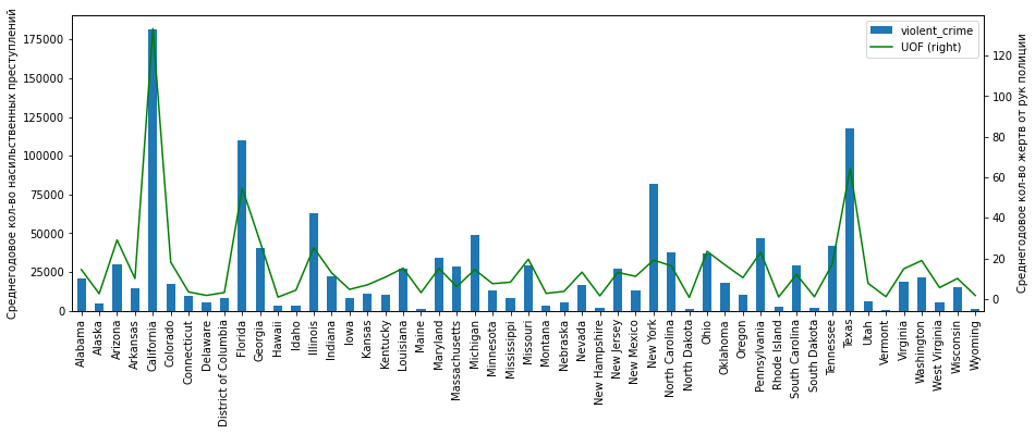
, :
" ": "" ;
(, , , -, ) ( ) .
:
plt = df_fenc_crime_states_agg.plot.scatter(x='violent_crime', y='UOF')
plt.set_xlabel(' -  ')
plt.set_ylabel(' -    ')
, . , 75 . , 75 . "" , , . " ":
df_fenc_crime_states_agg[df_fenc_crime_states_agg['violent_crime'] > 75000]UOF | violent_crime | |
|---|---|---|
state_name | ||
California | 133.263158 | 181514.578947 |
Florida | 54.578947 | 110104.315789 |
New York | 19.157895 | 81618.052632 |
Texas | 64.368421 | 117614.631579 |
, " ": , , -.
3 :
75 .
75 . ( "")
:
df_fenc_crime_states_agg[df_fenc_crime_states_agg['violent_crime'] <= 75000].corr(method='pearson').at['UOF', 'violent_crime']0.839. , 0.9 , 47 .
:
df_fenc_crime_states_agg[df_fenc_crime_states_agg['violent_crime'] > 75000].corr(method='pearson').at['UOF', 'violent_crime']0.999 - !
( ):
df_fenc_crime_states_agg.corr(method='pearson').at['UOF', 'violent_crime']: 0.935. .
, " " (, , ). , , :
df_fenc_crime_states_agg['uof_by_crime'] = df_fenc_crime_states_agg['UOF'] / df_fenc_crime_states_agg['violent_crime']
plt = df_fenc_crime_states_agg.loc[:, 'uof_by_crime'].sort_values(ascending=False).plot.bar(figsize=(15,5))
plt.set_xlabel('')
plt.set_ylabel(' -    - ')
, , , "" ( ).
:
1. (, !)
2. - : , , -.
2. ( ) , , - (. ).
3. , 0.93 . (.. ), - 0.84.
, , , . , , , . , , , , . . , (, , ), .
CSV :
ARRESTS_FILE = ROOT_FOLDER + '\\arrests_by_state_race.csv'
#
df_arrests = pd.read_csv(ARRESTS_FILE, sep=';', header=0, usecols=['data_year', 'state', 'white', 'black'])
#    4
df_arrests = df_arrests.groupby(['data_year', 'state']).sum().reset_index()
#
df_arrests = df_arrests.merge(df_state_names, left_on='state', right_on='state_abbr')
#
df_arrests = df_arrests.rename(columns={'data_year': 'year'}).drop(columns='state_abbr')
# ,
df_arrests.head()
year | state | black | white | state_name | |
|---|---|---|---|---|---|
0 | 2000 | AK | 140 | 613 | Alaska |
1 | 2001 | AK | 139 | 718 | Alaska |
2 | 2002 | AK | 143 | 677 | Alaska |
3 | 2003 | AK | 173 | 801 | Alaska |
4 | 2004 | AK | 163 | 765 | Alaska |
:
df_arrests_agg = df_arrests.groupby(['state_name']).mean().drop(columns='year')51 ( )
black | white | |
|---|---|---|
state_name | ||
Alabama | 2805.842105 | 1757.315789 |
Alaska | 221.894737 | 844.157895 |
Arizona | 1378.368421 | 7007.157895 |
Arkansas | 2387.894737 | 2303.789474 |
California | 26668.368421 | 87252.315789 |
Colorado | 1268.210526 | 5157.368421 |
Connecticut | 2097.631579 | 2981.210526 |
Delaware | 1356.894737 | 1048.578947 |
District of Columbia | 111.111111 | 4.944444 |
Florida | 12.000000 | 7.000000 |
Georgia | 8262.842105 | 3502.894737 |
Hawaii | 81.052632 | 368.736842 |
Idaho | 44.000000 | 1362.263158 |
Illinois | 5699.842105 | 1841.894737 |
Indiana | 3553.368421 | 5192.263158 |
Iowa | 1104.421053 | 3039.473684 |
Kansas | 522.315789 | 1501.315789 |
Kentucky | 1476.894737 | 1906.052632 |
Louisiana | 5928.789474 | 3414.263158 |
Maine | 63.736842 | 699.526316 |
Maryland | 7189.105263 | 4010.684211 |
Massachusetts | 3407.157895 | 7319.684211 |
Michigan | 7628.157895 | 6304.157895 |
Minnesota | 2231.210526 | 2645.736842 |
Mississippi | 1462.210526 | 474.368421 |
Missouri | 5777.473684 | 5703.368421 |
Montana | 27.684211 | 673.684211 |
Nebraska | 591.421053 | 1058.526316 |
Nevada | 1956.421053 | 3817.210526 |
New Hampshire | 68.368421 | 640.789474 |
New Jersey | 6424.157895 | 6043.789474 |
New Mexico | 234.421053 | 2809.368421 |
New York | 8394.526316 | 8734.947368 |
North Carolina | 10527.947368 | 7412.947368 |
North Dakota | 61.263158 | 277.052632 |
Ohio | 4063.947368 | 4071.368421 |
Oklahoma | 1625.105263 | 3353.000000 |
Oregon | 445.105263 | 3373.368421 |
Pennsylvania | 11974.157895 | 11039.473684 |
Rhode Island | 275.684211 | 699.210526 |
South Carolina | 5578.526316 | 3615.421053 |
South Dakota | 67.105263 | 349.368421 |
Tennessee | 6799.894737 | 8462.526316 |
Texas | 10547.631579 | 22062.684211 |
Utah | 167.105263 | 1748.894737 |
Vermont | 43.526316 | 439.210526 |
Virginia | 4100.421053 | 3060.263158 |
Washington | 1688.947368 | 6012.105263 |
West Virginia | 271.263158 | 1528.315789 |
Wisconsin | 3440.055556 | 4107.722222 |
Wyoming | 27.263158 | 506.947368 |
. , - . , , - - 19 (12 7 ). - ; :
df_arrests[df_arrests['state'] == 'FL'], , , 2017 . , , ... . 1-2 . ( ) .
, ( 2000 2009 .) . , 9 ( 2010 2018 .).
POP_STATES_FILES = ROOT_FOLDER + '\\us_pop_states_race_2010-2019.csv'
df_pop_states = pd.read_csv(POP_STATES_FILES, sep=';', header=0)
#    ,   ))
df_pop_states = df_pop_states.melt('state_name', var_name='r_year', value_name='pop')
df_pop_states['race'] = df_pop_states['r_year'].str[0]
df_pop_states['year'] = df_pop_states['r_year'].str[2:].astype('uint16')
df_pop_states.drop(columns='r_year', inplace=True)
df_pop_states = df_pop_states[df_pop_states['year'].between(2000, 2018)]
df_pop_states = df_pop_states.groupby(['state_name', 'year', 'race']).sum().unstack().reset_index()
df_pop_states.columns = ['state_name', 'year', 'black_pop', 'white_pop']
state_name | year | black_pop | white_pop | |
|---|---|---|---|---|
0 | Alabama | 2010 | 5044936 | 13462236 |
1 | Alabama | 2011 | 5067912 | 13477008 |
2 | Alabama | 2012 | 5102512 | 13484256 |
3 | Alabama | 2013 | 5137360 | 13488812 |
4 | Alabama | 2014 | 5162316 | 13493432 |
... | ... | ... | ... | ... |
454 | Wyoming | 2014 | 31392 | 2167008 |
455 | Wyoming | 2015 | 29568 | 2177740 |
456 | Wyoming | 2016 | 29304 | 2170700 |
457 | Wyoming | 2017 | 29444 | 2148128 |
458 | Wyoming | 2018 | 29604 | 2139896 |
1 :
df_arrests_2010_2018 = df_arrests.merge(df_pop_states, how='inner', on=['year', 'state_name'])
df_arrests_2010_2018['white_arrests_promln'] = df_arrests_2010_2018['white'] * 1e6 / df_arrests_2010_2018['white_pop']
df_arrests_2010_2018['black_arrests_promln'] = df_arrests_2010_2018['black'] * 1e6 / df_arrests_2010_2018['black_pop']
:
df_arrests_2010_2018_agg = df_arrests_2010_2018.groupby(['state_name', 'state']).mean().drop(columns='year').reset_index()
df_arrests_2010_2018_agg = df_arrests_2010_2018_agg.set_index('state_name')
( )
state | black | white | black_pop | white_pop | white_arrests_promln | black_arrests_promln | |
|---|---|---|---|---|---|---|---|
state_name | |||||||
Alabama | AL | 1682.000000 | 1342.000000 | 5.152399e+06 | 1.349158e+07 | 99.424741 | 324.055203 |
Alaska | AK | 255.000000 | 870.555556 | 1.069489e+05 | 1.957445e+06 | 445.199704 | 2390.243876 |
Arizona | AZ | 1635.555556 | 6852.000000 | 1.279172e+06 | 2.260403e+07 | 302.923002 | 1267.000192 |
Arkansas | AR | 1960.666667 | 2466.000000 | 1.855574e+06 | 9.465137e+06 | 260.459917 | 1055.854934 |
California | CA | 24381.666667 | 79477.000000 | 1.007921e+07 | 1.128020e+08 | 704.731408 | 2419.234376 |
Colorado | CO | 1377.222222 | 5171.555556 | 9.508173e+05 | 1.882940e+07 | 274.209456 | 1439.257054 |
Connecticut | CT | 1823.777778 | 2295.333333 | 1.643690e+06 | 1.165681e+07 | 196.712775 | 1114.811569 |
Delaware | DE | 1318.000000 | 914.111111 | 8.354622e+05 | 2.635794e+06 | 347.374980 | 1582.395733 |
District of Columbia | DC | 139.222222 | 4.777778 | 1.288488e+06 | 1.154416e+06 | 4.112547 | 108.101938 |
Florida | FL | 12.000000 | 7.000000 | 1.415383e+07 | 6.498292e+07 | 0.107721 | 0.847827 |
Georgia | GA | 8137.222222 | 4271.444444 | 1.279378e+07 | 2.500293e+07 | 170.939250 | 639.869143 |
Hawaii | HI | 81.333333 | 383.777778 | 1.124298e+05 | 1.453712e+06 | 264.353469 | 725.477589 |
Idaho | ID | 51.888889 | 1373.777778 | 5.288222e+04 | 6.154316e+06 | 223.151878 | 978.205026 |
Illinois | IL | 4216.000000 | 1284.222222 | 7.554687e+06 | 3.980927e+07 | 32.199075 | 557.493894 |
Indiana | IN | 2924.444444 | 5186.111111 | 2.522917e+06 | 2.267508e+07 | 228.699515 | 1155.168768 |
Iowa | IA | 1181.000000 | 2999.222222 | 4.305640e+05 | 1.141794e+07 | 262.666753 | 2760.038539 |
Kansas | KS | 539.555556 | 1512.111111 | 7.116182e+05 | 1.006714e+07 | 150.232160 | 758.851182 |
Kentucky | KY | 1443.888889 | 2173.666667 | 1.442174e+06 | 1.558094e+07 | 139.526970 | 1001.433470 |
Louisiana | LA | 5917.000000 | 3255.333333 | 6.021228e+06 | 1.174245e+07 | 277.277874 | 981.334817 |
Maine | ME | 78.000000 | 678.000000 | 7.667733e+04 | 5.059062e+06 | 134.024032 | 1019.061684 |
Maryland | MD | 6460.444444 | 3325.444444 | 7.229037e+06 | 1.426036e+07 | 233.317775 | 893.942720 |
Massachusetts | MA | 3349.555556 | 6895.111111 | 2.249232e+06 | 2.226671e+07 | 309.745910 | 1505.096888 |
Michigan | MI | 6302.444444 | 5647.444444 | 5.645176e+06 | 3.170670e+07 | 178.111684 | 1116.364030 |
Minnesota | MN | 2570.000000 | 2686.777778 | 1.311818e+06 | 1.867259e+07 | 143.902882 | 1986.464052 |
Mississippi | MS | 1251.000000 | 418.777778 | 4.478208e+06 | 7.122651e+06 | 58.753686 | 279.574565 |
Missouri | MO | 4588.333333 | 5146.111111 | 2.854060e+06 | 2.023871e+07 | 254.292323 | 1608.303611 |
Montana | MT | 34.222222 | 788.333333 | 2.210444e+04 | 3.660813e+06 | 214.944902 | 1525.795754 |
Nebraska | NE | 618.888889 | 1154.888889 | 3.701520e+05 | 6.709768e+06 | 172.269972 | 1687.725359 |
Nevada | NV | 2450.000000 | 4480.333333 | 1.052192e+06 | 8.647157e+06 | 517.401564 | 2316.374085 |
New Hampshire | NH | 89.777778 | 784.777778 | 7.873600e+04 | 5.012056e+06 | 156.580888 | 1141.127571 |
New Jersey | NJ | 5429.555556 | 4971.888889 | 5.241910e+06 | 2.595141e+07 | 191.427955 | 1037.217679 |
New Mexico | NM | 260.111111 | 3136.000000 | 2.053876e+05 | 6.905377e+06 | 454.129135 | 1268.115549 |
New York | NY | 6035.777778 | 6600.222222 | 1.373077e+07 | 5.534157e+07 | 119.253616 | 439.581451 |
North Carolina | NC | 9549.000000 | 6759.333333 | 8.804027e+06 | 2.844145e+07 | 238.320077 | 1088.968561 |
North Dakota | ND | 100.666667 | 386.222222 | 6.583289e+04 | 2.583206e+06 | 149.190455 | 1536.987272 |
Ohio | OH | 3632.888889 | 3733.333333 | 5.879375e+06 | 3.844592e+07 | 97.107129 | 617.699379 |
Oklahoma | OK | 1577.333333 | 3049.000000 | 1.189604e+06 | 1.160567e+07 | 262.904593 | 1326.463864 |
Oregon | OR | 375.444444 | 3125.000000 | 3.292284e+05 | 1.402225e+07 | 222.819615 | 1148.158169 |
Pennsylvania | PA | 11227.000000 | 10652.111111 | 5.945100e+06 | 4.232445e+07 | 251.598838 | 1893.415475 |
Rhode Island | RI | 274.888889 | 595.000000 | 3.275551e+05 | 3.592825e+06 | 165.605635 | 837.932682 |
South Carolina | SC | 4703.222222 | 3094.111111 | 5.365012e+06 | 1.324712e+07 | 234.287821 | 877.892998 |
South Dakota | SD | 103.777778 | 448.333333 | 6.154533e+04 | 2.903489e+06 | 153.995184 | 1641.137012 |
Tennessee | TN | 7603.000000 | 9068.666667 | 4.460808e+06 | 2.070126e+07 | 438.486812 | 1708.022356 |
Texas | TX | 10821.666667 | 21122.111111 | 1.345661e+07 | 8.628389e+07 | 245.051258 | 803.917061 |
Utah | UT | 193.222222 | 1797.333333 | 1.558876e+05 | 1.079659e+07 | 166.431266 | 1240.117890 |
Vermont | VT | 54.222222 | 520.555556 | 3.017111e+04 | 2.376143e+06 | 219.129918 | 1785.111547 |
Virginia | VA | 4059.555556 | 3071.222222 | 6.544598e+06 | 2.340732e+07 | 131.178648 | 620.504151 |
Washington | WA | 1791.777778 | 5870.444444 | 1.147000e+06 | 2.289368e+07 | 256.632241 | 1566.862244 |
West Virginia | WV | 294.111111 | 1648.666667 | 2.597649e+05 | 6.908718e+06 | 238.517207 | 1132.059057 |
Wisconsin | WI | 3525.333333 | 4046.222222 | 1.516534e+06 | 2.018658e+07 | 200.441064 | 2325.622492 |
Wyoming | WY | 28.777778 | 464.555556 | 2.856356e+04 | 2.151349e+06 | 216.004646 | 1005.725503 |
:
plt = df_arrests_2010_2018_agg.loc[:, ['white', 'black']].sort_index(ascending=False).plot.barh(color=['g', 'olive'], figsize=(10, 20))
plt.set_ylabel('')
plt.set_xlabel(' -  (2010-2018 .)')

2. :
plt = df_arrests_2010_2018_agg.loc[:, ['white_arrests_promln', 'black_arrests_promln']].sort_index(ascending=False).plot.barh(color=['g', 'olive'], figsize=(10, 20))
plt.set_ylabel('')
plt.set_xlabel(' -   1    (2010-2018 .)')
?
-, , - .
-, . "", , (. , , , .) -, ( , , , , , .
-, ( ) , .
.
:
df_arrests_2010_2018['white'].mean() / df_arrests_2010_2018['black'].mean()- 1.56. .. 9 , .
:
df_arrests_2010_2018['white_arrests_promln'].mean() / df_arrests_2010_2018['black_arrests_promln'].mean()- 0.183. .. 5.5 , .
, .
, , .
:
df_fenc_agg_states1 = df_fenc.merge(df_state_names, how='inner', left_on='State', right_on='state_abbr')
df_fenc_agg_states1.fillna(0, inplace=True)
df_fenc_agg_states1 = df_fenc_agg_states1.rename(columns={'state_name_x': 'state_name', 'Year': 'year'})
df_fenc_agg_states1 = df_fenc_agg_states1.loc[df_fenc_agg_states1['year'].between(2000, 2018), ['year', 'Race', 'state_name', 'UOF']]
df_fenc_agg_states1 = df_fenc_agg_states1.groupby(['year', 'state_name', 'Race'])['UOF'].count().unstack().reset_index()
df_fenc_agg_states1 = df_fenc_agg_states1.rename(columns={'Black': 'black_uof', 'White': 'white_uof'})
df_fenc_agg_states1 = df_fenc_agg_states1.fillna(0).astype({'black_uof': 'uint32', 'white_uof': 'uint32'})
year | state_name | black_uof | white_uof | |
|---|---|---|---|---|
0 | 2000 | Alabama | 4 | 3 |
1 | 2000 | Alaska | 0 | 2 |
2 | 2000 | Arizona | 0 | 11 |
3 | 2000 | Arkansas | 1 | 3 |
4 | 2000 | California | 19 | 78 |
... | ... | ... | ... | ... |
907 | 2018 | Virginia | 11 | 7 |
908 | 2018 | Washington | 0 | 24 |
909 | 2018 | West Virginia | 2 | 5 |
910 | 2018 | Wisconsin | 3 | 7 |
911 | 2018 | Wyoming | 0 | 4 |
:
df_arrests_fenc = df_arrests.merge(df_fenc_agg_states1, on=['state_name', 'year'])
df_arrests_fenc = df_arrests_fenc.rename(columns={'white': 'white_arrests', 'black': 'black_arrests'})
2017
year | state | black_arrests | white_arrests | state_name | black_uof | white_uof | |
|---|---|---|---|---|---|---|---|
15 | 2017 | AK | 266 | 859 | Alaska | 2 | 3 |
34 | 2017 | AL | 3098 | 2509 | Alabama | 7 | 17 |
53 | 2017 | AR | 2092 | 2674 | Arkansas | 6 | 7 |
72 | 2017 | AZ | 2431 | 7829 | Arizona | 6 | 43 |
91 | 2017 | CA | 24937 | 80367 | California | 25 | 137 |
110 | 2017 | CO | 1781 | 6079 | Colorado | 2 | 27 |
127 | 2017 | CT | 1687 | 2114 | Connecticut | 1 | 5 |
140 | 2017 | DE | 1198 | 782 | Delaware | 4 | 3 |
159 | 2017 | GA | 7747 | 4171 | Georgia | 15 | 21 |
173 | 2017 | HI | 88 | 419 | Hawaii | 0 | 1 |
192 | 2017 | IA | 1400 | 3524 | Iowa | 1 | 5 |
210 | 2017 | ID | 61 | 1423 | Idaho | 0 | 6 |
229 | 2017 | IL | 2847 | 947 | Illinois | 13 | 11 |
248 | 2017 | IN | 3565 | 4300 | Indiana | 9 | 13 |
267 | 2017 | KS | 585 | 1651 | Kansas | 3 | 10 |
286 | 2017 | KY | 1481 | 2035 | Kentucky | 1 | 18 |
305 | 2017 | LA | 5875 | 2284 | Louisiana | 13 | 5 |
324 | 2017 | MA | 2953 | 6089 | Massachusetts | 1 | 4 |
343 | 2017 | MD | 6662 | 3371 | Maryland | 8 | 5 |
361 | 2017 | ME | 89 | 675 | Maine | 1 | 8 |
380 | 2017 | MI | 6149 | 5459 | Michigan | 6 | 7 |
399 | 2017 | MN | 2513 | 2681 | Minnesota | 1 | 7 |
418 | 2017 | MO | 4571 | 5007 | Missouri | 13 | 20 |
437 | 2017 | MS | 1266 | 409 | Mississippi | 7 | 10 |
455 | 2017 | MT | 50 | 915 | Montana | 0 | 3 |
474 | 2017 | NC | 8177 | 5576 | North Carolina | 9 | 14 |
501 | 2017 | NE | 80 | 578 | Nebraska | 0 | 1 |
516 | 2017 | NH | 113 | 817 | New Hampshire | 0 | 3 |
535 | 2017 | NJ | 4859 | 4136 | New Jersey | 9 | 6 |
554 | 2017 | NM | 205 | 2094 | New Mexico | 0 | 20 |
573 | 2017 | NV | 2695 | 4657 | Nevada | 3 | 12 |
592 | 2017 | NY | 5923 | 6633 | New York | 7 | 9 |
611 | 2017 | OH | 4472 | 3882 | Ohio | 11 | 23 |
630 | 2017 | OK | 1638 | 2872 | Oklahoma | 3 | 20 |
649 | 2017 | OR | 453 | 3222 | Oregon | 2 | 9 |
668 | 2017 | PA | 10123 | 10191 | Pennsylvania | 7 | 17 |
681 | 2017 | RI | 315 | 633 | Rhode Island | 0 | 1 |
700 | 2017 | SC | 4645 | 2964 | South Carolina | 3 | 10 |
712 | 2017 | SD | 124 | 537 | South Dakota | 0 | 2 |
731 | 2017 | TN | 6654 | 8496 | Tennessee | 4 | 24 |
750 | 2017 | TX | 11493 | 20911 | Texas | 18 | 56 |
769 | 2017 | UT | 199 | 1964 | Utah | 1 | 5 |
788 | 2017 | VA | 4283 | 3247 | Virginia | 8 | 17 |
804 | 2017 | VT | 75 | 626 | Vermont | 0 | 1 |
823 | 2017 | WA | 1890 | 5804 | Washington | 8 | 27 |
842 | 2017 | WV | 350 | 1705 | West Virginia | 1 | 10 |
856 | 2017 | WY | 36 | 549 | Wyoming | 0 | 1 |
872 | 2017 | DC | 135 | 8 | District of Columbia | 1 | 1 |
890 | 2017 | WI | 3604 | 4106 | Wisconsin | 6 | 15 |
892 | 2017 | FL | 12 | 7 | Florida | 19 | 43 |
, , :
df_corr = df_arrests_fenc.loc[:, ['white_arrests', 'black_arrests', 'white_uof', 'black_uof']].corr(method='pearson').iloc[:2, 2:]
df_corr.style.background_gradient(cmap='PuBu')
white_uof | black_uof | |
|---|---|---|
white_arrests | 0.872766 | 0.622167 |
black_arrests | 0.702350 | 0.766852 |
: 0.87 0.77 ! , , ( 0.88 0.72 ).
, " ", :
df_arrests_fenc['white_uof_by_arr'] = df_arrests_fenc['white_uof'] / df_arrests_fenc['white_arrests']
df_arrests_fenc['black_uof_by_arr'] = df_arrests_fenc['black_uof'] / df_arrests_fenc['black_arrests']
df_arrests_fenc.replace([np.inf, -np.inf], np.nan, inplace=True)
df_arrests_fenc.fillna({'white_uof_by_arr': 0, 'black_uof_by_arr': 0}, inplace=True)
, ( 2018 ):
plt = df_arrests_fenc.loc[df_arrests_fenc['year'] == 2018, ['state_name', 'white_uof_by_arr', 'black_uof_by_arr']].sort_values(by='state_name', ascending=False).plot.barh(x='state_name', color=['g', 'olive'], figsize=(10, 20))
plt.set_ylabel('')
plt.set_xlabel(' -   -  ( 2018 .)')
, , : , , , .
:
plt = df_arrests_fenc.loc[:, ['white_uof_by_arr', 'black_uof_by_arr']].mean().plot.bar(color=['g', 'olive'])
plt.set_ylabel(' -   - ')
plt.set_xticklabels(['', ''], rotation=0)
2.5 . , - , 2.5 , . , : , 2 , - 4 .
, . .
. "" , , - . ( ) - , ( ) -.
( ), .
: 3 5 , .
2.5 , .
: , . , . : , .
, :)
PS. In the next, separate article, I plan to continue looking at crime in the United States and its relationship to race. First, let's play with the official data on crimes motivated by racial and other intolerance, and then we will look at the conflicts between the police and the population from the other side and analyze the cases of police deaths in the line of duty. If this topic is interesting, please let me know in the comments!
Link to the English version of the article (at the request of workers).