Reed-Solomon code

An important task of codology in the processing of information streams of encoded messages in the channels of communication systems and computer is the separation of streams and their selection according to the given features. The dedicated stream is split into separate messages and for each of them an in-depth analysis is performed in order to establish the code and its characteristics, followed by decoding and access to the semantics of the message.



So, for example, for a certain Reed-Solomon code (PC code), you need to set:

• the length n of the codeword (block);
• the number of k information and Nk check symbols;
• an irreducible polynomial p (x) defining a finite field GF (2 ^r );
• primitive element α of a finite field;
• generating polynomial g (x);
• parameter j of the code;
• used interleaving;
• sequence of transmission of codewords or symbols to the channel and some others.

Here, a slightly different particular problem is considered in the work - modeling of the PC code itself, which is the central main part of the above-mentioned code analysis problem.

Description of the PC-code and its characteristics

For convenience and a better understanding of the essence of the PC-code device and the coding process, we first present the basic concepts and terms (elements) of the code.



Reed - Solomon codes (RS code) can be interpreted as non-binary BCH codes (Bose - Chowdhury - Hawkingham), the values ​​of the code symbols of which are taken from the GF (2 ^r ) field , i.e. r information symbols are displayed as a separate element of the field. Reed-Solomon codes are linear non-binary systematic cyclic codes whose symbols are r-bit sequences, where r is a positive integer greater than 1.



Reed-Solomon codes (n, k) are defined on r-bit symbols for all n and k, for which:

0 <k <n <2 ^r + 2, where

k is the number of information symbols to be encoded,

n is the number of code symbols in the coded block.



For most (n, k) -codes of Reed - Solomon; (n, k) = (2 ^r –1, 2 ^r –1–2 ∙ t), where

t is the number of erroneous symbols that the code can correct, and

n – k = 2t is the number of check symbols.



The Reed-Solomon code has the largest minimum distance (the number of characters that distinguish the sequences) possible for a linear code. For Reed - Solomon codes, the minimum distance is defined as follows: dmin = n – k +1.



Definition . PC code over the field GF (q = ^m ), with block length n = q ^m-1, correcting t errors, is the set of all codewords u _(n) over GF (q) for which 2t consecutive spectrum components with numbers$$$m_0,m_0 +1,...,m_0+2t-1$equal to 0.



The fact that 2t consecutive powers of α are roots of the generating polynomial g (x) or that the spectrum contains 2t consecutive zero components is an important property of the code that allows t errors to be corrected.



Information polynomial Q. Specifies the text of the message, which is divided into blocks (words) of constant length and digitized. This is what is to be transmitted in the communication system.

Generating polynomial g (x) of a PC code is a polynomial that transforms information polynomials (messages) into code words by multiplying Q · g (x) = = u _(n) over GF (q).



The check polynomial h (x) allows you to establish the presence of distorted characters in a word.

Syndrome polynomialS (z). A polynomial containing components corresponding to erroneous positions. Computed for each word received by the decoder.

Error polynomial E. A polynomial with a length equal to the codeword, with zero values ​​in all positions, except for those that contain distortions of the codeword symbols.



The error locator polynomial Λ (z) provides roots that indicate the error positions in words received by the receiving side of the communication channel (decoder). Its roots can be found by trial and error, i.e. by substituting in turn all the elements of the field until Λ (z) becomes equal to zero.

The polynomial of error values Ω (z) ≡Λ (z) S (z) (modz ^2t ) is comparable modulo z ^2twith the product of the error locator polynomial by the syndromic polynomial.



Irreducible polynomial of the field p (x). Finite fields do not exist for any number of elements, but only if the number of elements is a prime number p or a power q = p ^{m of a} prime number. In the first case, the field is called simple (its elements are the residue of numbers modulo a prime p), in the second, it is an extension of the corresponding prime field (its q elements of polynomials of degree m-1 or less are the residues of polynomials modulo the polynomial p (x) of degree m)



Primitive polynomial . If the root of an irreducible polynomial of the field is a primitive element α, then p (x) is called an irreducible primitive polynomial.



In the course of describing actions with the PC code, we will need to repeatedly refer to the Galois field, therefore, immediately here we will place a worksheet with the elements of this field with different representations of the elements (decimal number, binary vector, polynomial, degree of a primitive element ).



Table II - Characteristics of elements of the finite field of the extension GF (2 ⁴ ), irreducible polynomial p (x) = x ⁴ + x + 1, primitive element α = 0010 = 2 ₁₀





Example 1 . Over a finite field GF (2 ⁴ ), an irreducible field polynomial p (x) = x ⁴ + x + 1 is given, a primitive element α = 2, and an (n, k) - Reed-Solomon code (PC-code) is given. The code distance of this code is d = n - k + 1 = 7. This code can correct up to three errors in the block (code word) of the message.



The generating polynomial g (z) of the code has degree m = nk = 15-9 = 6 (its roots are 6 elements of the field GF (2 ⁴ ) in decimal notation, namely, elements 2, 3, 4, 5, 6, 7) and is determined by the ratio, i.e. polynomial in z with coefficients (elements) from GF (2 ⁴ ) in decimal representation for i = 1 (1) 6. In the considered PC-code 2 ⁹ = 512 codewords.

PC message encoding

In table II, these roots also have a power representation $$$α^1=2, α^2=3,...,α^6=7$...





Here z is an abstract variable, and α is a primitive element of the field, through its powers all (16) elements of the field are expressed. The polynomial representation of field elements uses the x variable.

The calculation of the generating polynomial g (x) = A B of the PC code is performed in parts (three brackets each):





The vector representation (through the coefficients g (z) by the field elements in decimal representation) of the generating polynomial has the form



g (z) = G _<7> = (1, 11, 15, 5, 7, 10, 7).



After the generation of the generating polynomial of the PC-code oriented towards error detection and correction, a message is set. The message is presented in digital form (for example, ASCII code), from which the transition to polynomial or vector representation.



An information vector (message word) has k - components from (n, k). In the example k = 9, the vector is 9-component, all components are elements of the GF field (2 ⁴ ) in decimal representation Q _<9> = (11, 13, 9, 6, 7, 15, 14, 12, 10) ...



From this vector, the code word u is formed_<15> is a vector with 15 components. Code words, like codes themselves, are systematic and non-systematic. A non-systematic codeword is obtained by multiplying the information vector Q by the vector corresponding to the generating polynomial



After transformations, we obtain a non-systematic codeword (vector) in the form

Q · g = <11, 15, 3, 9, 6, 14, 7, 5, 12, 15, 14, 3, 3, 7, 1>.



In systematic coding, a message (information vector) is represented by a polynomial Q (z) in the form Q (z) = q (z) g (z) + R (z), where the degree degR (z) <m = 6. After that, to the vector Q on the right is assigned the remainder R (all in decimal form). This is done like this.



The polynomial Q is shifted towards the higher digits by the value m = n - k, which is achieved by multiplying Q (z) by Z ^{n - k} (in the example Z ^{n - k} = Z ⁶ ) and after the shift, the division Q (z) Z ^{n - k} by g (z). As a result, find the remainder of the division R (z). All operations are performed on the GF field (2 ⁴ )



(11, 13, 9, 6, 7, 15, 14, 12, 10, 0, 0, 0, 0, 0, 0) =

= (1, 11, 15, 5, 7, 10, 7) ( 11, 15, 9, 10,12,10,10,10,10,3) + (1, 2, 3, 7, 13, 9) = G · S + R.



The remainder of the division of polynomials is calculated in the usual way ( see corner here Example 6 ). The division is performed according to the pattern: Let Q = 26, g (z) = 7 then 26 = 7 3 + R (z), R (z) = 26 -7 3 = 26-21 = 5. Calculation of the remainder R (z ) on the division of polynomials. We assign the remainder R to the vector Q on the right.



We get u _<15> - a code word in a systematic form. This view clearly contains an information message in the k high- order bits of the codeword



u _<15> = (11,13,9,6,7,15,14,12,10; 1, 2, 3, 7, 13, 9)



The digits of the vector are numbered from right to left from 0 (1) 14. The six least significant bits on the right are the check ones.

Decoding Reed-Solomon codes

After receiving a block, the decoder processes each block (codeword) and corrects errors that occurred during transmission or storage. The decoder divides the resulting polynomial by the generating polynomial of the RS code. If the remainder is zero, then no errors were found, otherwise, errors occur.



A typical PC decoder performs five steps in a decoding loop, namely:

1. Calculation of the syndromic polynomial (its coefficients), errors are found.
2. The key Pade equation is solved - calculating the error values ​​and their positions of the corresponding locations.
3. Chen's procedure is implemented - finding the roots of the error locator polynomial.
4. Forney's algorithm is used to calculate the error value.
5. Corrections are made to distorted codewords;

The cycle ends by extracting the message from the code words (removing the code).



Calculation of the syndrome.



Syndrome generation from the received codeword is the first step in the

decoding process . Here syndromes are calculated and it is determined whether there are errors in the received codeword or not. The



decoding of the PC code words can be organized in different ways. The classical methods include decoding using algorithms operating in the time or frequency domain, which either use the computation of the syndrome, or do not. Without delving into the theory of this issue, we will opt for decoding with the computation of codeword syndromes in the time domain.

Distortion detection

Syndromic $$$S = (S_v,S_{v+1},...,S_{m+v-1})$where $$$v∊{0, 1}$the vector is sequentially determined for each of the codewords received by the decoder at its input. With zero values ​​of the components of the syndrome vector$$$Sj = 0, j=v,v+1,...,m + v - 1$, the decoder considers that there is no error in the received word. If for at least one$$$j≥1,Sj≠0$, then the decoder concludes that there are errors in the code vector and proceeds to identify them, which is the first step in the decoder's operation.



Calculation of the syndromic polynomial

Multiplication on the receiving side of the codeword C by the parity-check matrix H can result in two outcomes:

• syndrome vector S = 0, which corresponds to the absence of errors in vector C;
• syndrome vector S ≠ 0, which means the presence of errors (one or more) in the components of vector C.

The second case is of interest.



The code vector with errors is represented as C (E) = C + E, E is the error vector. Then$$$(C +E)H^t = CH^t + EH^t = 0 + EH^t = S$



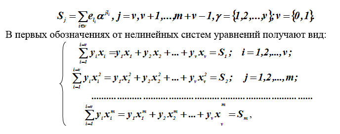
The components Sj of the syndrome are determined either by the summation relation

for n = q-1 and j = 1 (1) m = nk, or by Horner's scheme:



$$$S_j = C_0 +α^j(C_1 +α^j(C_2 +...+α^j(C_{n-2} +α^jC_{n-1})...))$



Example 2 . Let the error vector have the form = <0 0 0 0 12 0 0 0 0 0 0 8 0 0 0>. It mangles the characters at the 3rd and 10th positions in the code vector. The error values ​​are 8 and 12, respectively - these values ​​are also elements of the GF field (2 ⁴ ) and are given in decimal (Table P) notation. In vector E, the positions are numbered from lower ones from right to left, starting from 0 (1) 14.



Let us now form a code vector with two errors in the 3rd bit and in the 10th one with the values ​​8 and 12, respectively. This is done by summing in the GF (2 ⁴) according to the rules of arithmetic of this field. Summing field elements with zero does not change their value. Nonzero values ​​(field elements) are summed after converting them to a polynomial representation, as polynomials are usually summed, but the coefficients for the unknown are reduced mod 2.



After the summation result is obtained, they are again converted to decimal representation, having previously passed through the power representation





The following shows the calculation of error-corrupted values ​​at 10 and 3 positions of the codeword:



$$$(7+12) →α^6+α^11 =x^3 +x^2 +x^3 +x^2 +x^1 =α^1 = 2,$

$$$(3 + 8) →α^2+ α^7 =x^2 +x^3 +x^1 + 1 =α^{12}=13.$



The decoder performs calculations according to the general formula for the components Sj, j = 1 (1) m. Here (in the model) we use the relation$$$S=EH^t$, since we specify (simulate) in the program ourselves, nonzero terms are obtained only for i = 3 and i = 10.





Below, we will specially show the calculations by this formula in expanded form.

PC code check matrix

As soon as the generating polynomial of the code is formulated, it becomes possible to construct a check matrix for code words, as well as to determine the number of errors to be corrected ( see here, the decoder ). Let's construct an auxiliary matrix [7 × 15], from which two different parity check matrices can be obtained: the first six rows are one and the last six rows are the other.



The matrix itself is formed in a special way. The first two lines are obvious, the third line and all subsequent ones are obtained by subtracting from the previous (second) line a segment of natural numbers 1, 2, 3, 4, 5, 6, 7, 8, 9, 10, 11, 12, 13, 14, 15 mod 15. When a zero value occurs, it is replaced with 15, negative residues are converted to positive ones.





Each matrix corresponds to its own generator polynomial for systematic and non-systematic coding.

Determination of the coefficients of the syndromic polynomial

In what follows, we will determine the coefficients of the syndromic polynomial for j = 1 (1) 6.

With respect to a codeword with length$$$n<q=p^r$arriving at the input of the decoder, we assume that it is distorted by errors.



To identify the vector of errors, you need to know the following:

• the number of distorted positions in the code word
• $$$v≤v_{max}=0.5m$;
• numbers (position) of distorted positions in a codeword $$$ℓ_i: ℓ_i=0(1)n-1$;
• distortion values $$$e_ℓ; e_ℓ∊GF(2^4)$...

How is the syndrome vector (polynomial) S calculated and used further? Its role in decoding codewords is very significant. Let us show this with an illustration using a numerical example.



Example 3 . (Calculation of the components of the syndrome vector$$$S_{<6>}$ )





then in the end we have $$$S_{<6>}=(S_1,S_2,S_3,S_4,S_5,S_6)$= <8,13,7,13,15,15>



For further consideration, we introduce new concepts. The quantity$$$x_i = α^{ℓ_i}$will be called an error locator, here the distorted codeword symbol at the position $$$ℓ_i$, α is a primitive element of the field GF (2 ⁴ ).



The set of error locators for a specific codeword is considered below as the coefficients of the error locator polynomial σ (z), roots$$$z_i$ which are the values $$$x_i ^{-1}$inverse to locators.



Moreover, the expressions$$$(1-zx_i)=0$vanish.



$$$σ(z) = (1-zx_1)(1-zx_2)...(1-zx_v) =σ_vz^v +σ_{v-1}z^{v-1} +...+σ_1z +σ_0$

always free term of the equation always free term of the equation $$$σ_0 =1$...

The degree of the polynomial of error locators is equal to v - the number of errors and does not exceed the value$$$v≤v_{max}=0.5m$...



All distorted characters are in different positions of the word, therefore, among the locators$$$x_i = α^i$, there can be no repeated field elements, and the polynomial σ (z) = 0 has no multiple roots.



For convenience of writing, the error values ​​will be redesignated by the symbol$$$Y_i = e_i$... For the coefficients of the syndromic polynomial, nonlinear equations were previously considered. In our case, v = 1 is the origin of the components of the syndrome.





Where $$$y_i,x_i$ Are unknown quantities, and $$$S_j$- known, calculated at the first stage of decoding, parameters (components of the syndrome vector).



Methods for solving such systems of nonlinear equations are unknown, but solutions are found using tricks (workarounds). A transition is made to the Hankel (Toeplitz) system of linear equations for the coefficients$$$σ_i$the locator polynomial.



Conversion to a system of linear equations



To an equation$$$σ_i$ of the error locator polynomial, the value of its roots is substituted $$$z =x_i^{-1}$... In this case, the polynomial vanishes. An identity is formed, both sides of which are multiplied by$$$y_ix_i^{j+v}$, we get:



$$$y_i(σ_vx_i^{j}+σ_{v-1}x_i^{j+1}+...+σ_1x_i^{j+v-1}+x_i^{j+v})=0,1≤i≤v, 1≤j≤v$...



We obtain such equalities$$$v×v =v^2$



We sum these equalities over all $$$i, 1≤i≤v$for which these equalities are satisfied. Since the polynomial σ (z) has v roots$$$x_i^{-1}$, open the brackets and transfer the coefficients $$$σ_i$ per sign of the amount:





In this equality, according to the system of nonlinear equations given

earlier, each sum is equal to one of the components of the syndrome vector. Hence he concludes that with respect to the coefficients$$$σ_v, σ_{v-1},...,σ_1$ you can write out a system of linear equations.





Signs "-" when calculating over a binary field are omitted, since they correspond to "+". The resulting system of linear equations is Hankel and corresponds to a matrix with dimensions$$$v×(v+1)$ bit.





This matrix is ​​not degenerate if the number of errors in the codeword C (E) is strictly equal to $$$v , v ≤0.5(n-k)$, i.e. the noise immunity ability of this code is not violated.

Solving a system of linear equations

The resulting system of linear equations contains the coefficients as unknowns $$$σ_i =1(1)t$the error locator polynomial for the codeword C (E). The previously calculated components of the syndromic vector are considered known$$$S_j, j=1(1)m$... Here t is the number of errors in the word, m is the number of check positions in the word.



There are different methods for solving the formed system.



Note that the (Hankel) matrix is ​​not degenerate for dimensions limited by the number of errors allowed in a single word (less than 0.5m). In this case, the system of equations is uniquely solved, and the problem can be reduced simply to the inversion of the Hankel matrix. It would be desirable to remove the limitation on the dimension of matrices, i.e. over an endless field.



Methods for solving the Hankel system of linear equations are known over infinite fields:

• iterative Trench-Berlekamp-Messi method (TBM method); (1)
• direct deterministic Peterson - Gorenstein - Zierler; (PHC - method); (2)
• Sugiyama's method using Euclid's algorithm to find GCD (C-method). (3)

Without considering other methods, we will opt for the TBM method. The motivation for the choice is as follows.



The method (PHC) is simple and good, but for a small number of correctable errors, the C-method is difficult to implement on a computer and has been limitedly published (covered) in sources, although the C-method, like the TBM-method according to the well-known polynomial of syndromes S (z), provides solution of the Pade equation over the Galois field. This equation is formed for the polynomial of error locators σ (z) and the polynomial ω (z), in coding theory it is called the key Pade equation:



$$$S(z)σ(z) = ω(z)(mod z^m)$...



The solution to the key equation is the set$$$x_i^{-1}$ roots of the polynomial σ (z), and, accordingly, the locators $$$x_i =α^{ℓ_i}$, i.e. error positions. Error values ​​(magnitudes)$$$e_i$ are determined from the Forney formula in the form





Where $$$σ_z^{'}(α^{-i})$ and $$$ω(α^{-i})$ Are the values ​​of the polynomials σ (z) and ω (z) at the point $$$z =α^{-i}$inverse to the root of the polynomial σ (z);

i is the position of the error;$$$σ_z^{'}(z)$ - the formal derivative of the polynomial σ (z) with respect to z;

Formal derivative of a polynomial in a finite field

There are differences and similarities for the derivative with respect to a variable in the field of real numbers and the formal derivative in a finite field. Consider the polynomial





$$$a_i$Are the field elements, i = 1 (1) n



Field elements. A code over a real field GF (2 ⁴ ) is given. The derivative with respect to z is:





In an infinite real field, the operations multiply by n and sum n times coincide. For finite fields, the derivative is defined differently.



The derivative is similarly determined by the ratio:





where ((i)) = 1 + 1 + ... + 1, (i) times, summed according to the rules of a finite field: the + sign denotes the operation "sum up so many times", i.e. element$$$a_2z$ repeat 2 times, element $$$a_3z^2$ repeat 3 times, element $$$a_nz^{n-1}$repeat n times.



It is clear that this operation does not coincide with the operation of multiplication in a finite field. In particular, in the fields GF (2 ^r ), the sum of an even number of identical terms is taken mod2 and zeroed out, and an odd number is equal to the term itself without changes. Therefore, in the field GF (2 ^r ), the derivative takes the form





the second and highest even derivatives in this field are equal to zero.



It is known from algebra that if a polynomial has multiple roots (multiplicity p), then the derivative of the polynomial will have the same root, but with multiplicity p-1. If p = 1, then f (z) and f '(z) have no common root. Therefore, if a polynomial and its derivative have a common divisor, then there is a multiple root. All roots of the derivative f '(z) are multiples in f (z).

Key equation solution method

TMB (Trench-Berlekampa-Messi) is a method for solving the key equation. The iterative algorithm provides the definition of the polynomials σ (z) and ω (z), and the solution of the Pade (key) equation.



Initial data: polynomial coefficients$$$S_1,S_2,...,S_n$degree n-1.

Goal. Definition in explicit (analytic) form of the polynomials σ (z) and ω (z).



The algorithm uses the following notation: j - step number,$$$v_j$ - the degree of the polynomial, $$$σ_j(z) =σ_{ji}z^i +σ_{ji-1}z^{i-1}+...+σ_{j1}z+σ_{j0}$ - expansion of the polynomial in powers $$$z, k_j, L_j, θ_j(z)$ and $$$Ω_j(z)$- intermediate variables and functions at the j-th step of the algorithm;



The initial conditions must be specified, since recursion is used here.



Initial conditions:





Example 4 . Execution of an iterative algorithm for the vector

S = (8,13,7,13,15,15). Polynomials are defined$$$σ(z) =σ_n(z)$ and $$$ω(z) = ω_n(z)$...



Table 2 - Calculation of error locator polynomials







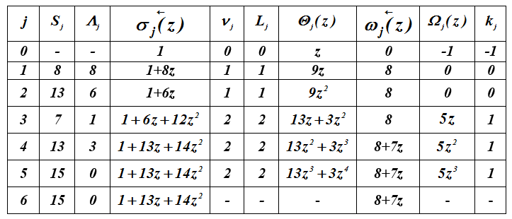
so $$$σ_j^←(z)=14z^2+13z+1$, $$$ω_j^←(z)$= 7z + 8.



The error locator polynomial σ (z) over the field GF (2 ⁴ ) with the irreducible polynomial p (x) = x ⁴ + x + 1 has roots



$$$z_1 = α^{-i_1} = 13 = 4^{-1}$ and $$$z_2 =α^{-i_2} = 6 = 11^{-1}$, it is easy to verify this by direct verification, i.e. $$$i_1= 3, i_2 =10, 13 = α^{12}, 1 =α^{12}α^{3}$ and $$$α^{12} =α^{-3}=>13=4^{-1}$... Root substitution in

$$$σ(z=13)=14(13)^2+13·13+1=α^{13}(α^{12})^2+(α^{12})^2+α^0= α^{37}+α^{24} +α^{0}$=

=$$$α^{7}+α^{9}+α^0 =x^3+x+1=0(mod2)$;

$$$σ(z = 6)=14(6)^2+13·6+1 = α^{13}(α^{5})^2+(α^{5})^2+α^{0}$=

=$$$α^{8}+α^{2} +α^{0} = x^2 +1+x^2 +1 = 0(mod2)$...



Taking the formal derivative of σ (z), we obtain σ_2 (z) = 2 14 + 13 = 13, since 14z is taken in the sum 2 times and vanishes mod 2.



Using the Forney formula, we will find expressions for calculating the error values$$$e_i$...



Substituting the values ​​i = 3 and i = 10 positions in the last expression,

we find



$$$_3 = 10α^{15-3}+11 =α^{6}+α^{10}$= =$$$x^3+x^2+x^2+x+1=x^3+x+1=α^{7}=>8$;

$$$_{10} = 10α^{15-10}+11 =α^{9}α^{5}+α^{10}=α^{14}+α^{10}$= =$$$x^3+x^2+x=α^{11}=>12$...

The architecture of building a software package

To build a software package, it is proposed to use the following architectural solution. The software package is implemented as an application with a graphical user interface.



The initial data for the software package is a digital stream of information unloaded using a dump from a file. For the convenience of analysis and clarity of the complex operation, it is supposed to use .txt files.



The loaded digital stream is presented in the form of data arrays, in the course of the complex work on which various computational actions are applied.



At each stage of the complex operation, it is possible to visualize the intermediate results of the work.



The results of the software package are presented in the form of numerical data displayed in tables.



The intermediate and final analysis results are saved to files.



Scheme of functioning of the software complex



Operation with the complex begins with loading a digital stream using a dump from a file. Once downloaded, the user is presented with a visual representation of the binary content of the file and its textual content.



Within the framework of this interface, the following functional tasks should be implemented:

• Download the original message;
• Converting a message to a dump;
• Message encoding;
• Simulating an intercepted message
• Construction of spectra of the received code words in order to analyze their visual representation;
• Displaying code parameters.

Description of the software package operation



When the executable file of the program is launched, the window shown in Figure 2 appears on the screen, in which the main interface of the program is displayed.



The input of the program is a file that needs to be transmitted over the communication channel. For its transmission over real communication channels, coding is required - the addition of check symbols to it, necessary for unambiguous decoding of a word at the source-receiver. To start the complex, you need to select the required text file using the “Load file” button. Its contents will be displayed in the lower field of the main program window.



The binary representation of the message will be presented in the corresponding field, the binary representation of information words - in the “Binary representation of information words” field.



The number of bits of the original message and the total number of words in it are displayed in the fields “Number of bits in the transmitted message” and “Number of words in the transmitted message”.



Formed information and code words are displayed in tables on the right side of the main program window.



The program window with intermediate results is shown in Figure 3.





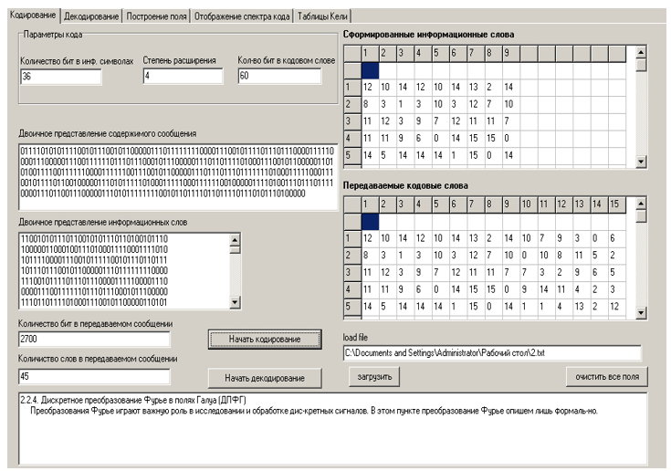
Figure 3 - Intermediate presentation of the results of the software package





Figure 4. Results of downloading the message file





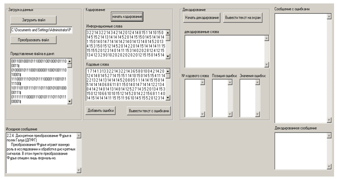
Figure 5. File encoding results





Figure 6. Output of a message with errors entered into it.





Figure 7. Output of the decoding results and the message with introduced errors.





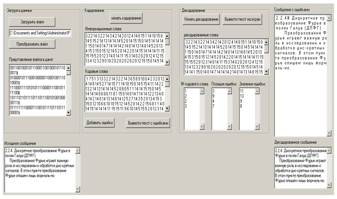
Figure 8. Output of the decoded message.

Conclusion

The US NSA is the primary operator of the Echelon global interception system. Echelon has an extensive infrastructure including ground tracking stations located all over the world. Almost all world information flows are monitored.



The study of the possibilities of gaining access to the semantics of encoded information messages at the present time of active information warfare both in the field of technology and in politics has become another challenge and one of the urgent and demanded tasks of our time.



In the overwhelming majority of codes, encoding and decoding of messages (information) is implemented on a rigorous mathematical basis of finite extended Galois fields. Working with elements of such fields differs from those generally accepted in arithmetic and requires, when using computational tools, writing special procedures for manipulating field elements.

The work offered to the readers' attention slightly opens the veil of secrecy over such activities at the level of firms, companies and states in general.