💆🏿 🤼 👨🏼‍🏫 We analyze the causal relationships of VK metrics 😜 🌝 🐶

Hello everyone, my name is Anver, I work in the Core ML VK team. One of our tasks is to create and improve ranking algorithms for news feed. In this article, I'll show you how you can use cause-and-effect analysis to help make the service more interesting for your users. Let's talk about the advantages of this approach over correlation analysis, and I will suggest modifications to existing algorithms.

What are short and long metrics?

Ranking models try to estimate the likelihood that the user will interact with the news (post): he will pay attention to it, put a mark “Like”, write a comment. The model then distributes the records in descending order of this probability. Therefore, by improving the ranking, we can get an increase in the CTR (click-through rate) of user actions: likes, comments, and others. These metrics are very sensitive to changes in the ranking model. I will call them short .

But there is another type of metrics. It is believed, for example, that the time spent in the application, or the number of user sessions, reflect much better his attitude to the service. We will call such metrics long .

Optimizing long metrics directly through ranking algorithms is not a trivial task. With short metrics, this is much easier: the CTR of likes, for example, is directly related to how well we estimate their likelihood. But if we know the causal (or causal) relationships between short and long metrics, then we can focus on optimizing only those short metrics that should predictably affect long ones. I tried to extract such causal connections - and wrote about it in my work, which I completed as a diploma at ITMO's Bachelor of Science (CT). We carried out the research in the Machine Learning laboratory of ITMO together with VKontakte.

Links to code, dataset and sandbox

You can find all the code here: AnverK .

To analyze the relationships between metrics, we used a dataset that includes the results of more than 6,000 real A / B tests that were conducted by the VK team at various times. The dataset is also available in the repository .

In the sandbox, you can see how to use the proposed wrapper: on synthetic data .

And here - how to apply algorithms to a dataset: on the proposed dataset .

Dealing with false correlations

It may seem that to solve our problem, it is enough to calculate the correlations between the metrics. But this is not entirely true: correlation is not always causation. Let's say we measure only four metrics and their causal relationships look like this:

Without loss of generality, let's assume that there is a positive influence in the direction of the arrow: the more likes, the more SPU. In this case, it will be possible to establish that comments on the photo have a positive effect on the SPU. And decide that if you "increase" this metric, the SPU will increase. This phenomenon is called false correlation.: The correlation coefficient is quite high, but there is no causal relationship. False correlations are not limited to two effects of the same cause. From the same graph, one could make the wrong conclusion that likes have a positive effect on the number of photo openings.

Even with such a simple example, it becomes obvious that a simple analysis of correlations will lead to many wrong conclusions. Causal inference (methods of inference of relationships) allows to restore causal relationships from data. To apply them in the task, we have chosen the most suitable causal inference algorithms, implemented python interfaces for them, and also added modifications of known algorithms that work better in our conditions.

Classical algorithms for inference links

We considered several methods of causal inference: PC (Peter and Clark), FCI (Fast Causal Inference) and FCI + (similar to FCI from a theoretical point of view, but much faster). You can read about them in detail in these sources:

Causality (J. Pearl, 2009),
Causation, Prediction and Search (P. Spirtes et al., 2000),
Learning Sparse Causal Models is not NP-hard (T. Claassen et al., 2013).

But it is important to understand that the first method (PC) assumes that we observe all quantities that affect two or more metrics - this hypothesis is called Causal Sufficiency. The other two algorithms take into account that there may be unobservable factors that affect the monitored metrics. That is, in the second case, the causal representation is considered more natural and allows the presence of unobservable factors

U_{1}, \dots U_{k}

$U_1, \dots U_k$ :

All implementations of these algorithms are provided in the pcalg library . It is beautiful and flexible, but with one "drawback" - it is written in R (when developing the most computationally heavy functions, the RCPP package is used). Therefore, for the above methods, I wrote wrappers in the CausalGraphBuilder class, adding examples of its use.

I will describe the contracts of the function of deriving links, that is, the interface and the result that can be obtained at the output. You can pass a test function for conditional independence. This is a test like this that returns

p_{v a l u e}

$p_{value}$ under the null hypothesis that the quantities

X

$X$ and

Y

$Y$ conditionally independent for a known set of quantities

Z

$Z$ ... The default is a partial correlation test . I chose the function with this test because it is the default in pcalg and is implemented in RCPP - this makes it fast in practice. You can also transfer

p_{v a l u e}

$p_{value}$ , starting from which the vertices will be considered dependent. For PC and FCI algorithms, you can also set the number of CPU cores, if you do not need to write a log of the library operation. There is no such option for FCI +, but I recommend using this particular algorithm - it wins in speed. Another caveat: FCI + currently does not support the proposed edge orientation algorithm - the point is in the limitations of the pcalg library.

Based on the results of the work of all algorithms, a PAG (partial ancestral graph) is built in the form of a list of edges. With the PC algorithm, it should be interpreted as a causal graph in the classical sense (or Bayesian network): an edge oriented from

A

$A$ at

B

$B$ , means influence

A

$A$ on

B

$B$ ... If the edge is non-directional or bidirectional, then we cannot uniquely orient it, which means:

or the available data is insufficient to establish a direction,
or it is impossible, because the true causal graph, using only observable data, can only be established up to an equivalence class.

The FCI algorithms will also result in PAG, but a new type of edges will appear in it - with an "o" at the end. This means that the arrow may or may not be there. In this case, the most important difference between FCI algorithms and PC is that a bidirectional (with two arrows) edge makes it clear that the vertices it connects are consequences of some unobservable vertex. Accordingly, a double edge in the PC algorithm now looks like an edge with two "o" ends. An illustration for such a case is in the sandbox with synthetic examples.

Modifying the edge orientation algorithm

The classical methods have one significant drawback. They admit that there may be unknown factors, but at the same time they rely on another overly serious assumption. Its essence is that the function of testing for conditional independence should be perfect. Otherwise, the algorithm is not responsible for itself and does not guarantee either the correctness or the completeness of the graph (the fact that more edges cannot be oriented without violating the correctness). Do you know many ideal finite sample conditional independence tests? Me not.

Despite this drawback, graph skeletons are built quite convincingly, but they are oriented too aggressively. So I suggested a modification to the edge orientation algorithm. Bonus: it allows you to implicitly adjust the number of oriented edges. To clearly explain its essence, it would be necessary to speak in detail here about the algorithms for the derivation of causal links. Therefore, I will attach the theory of this algorithm and the proposed modification separately - a link to the material will be at the end of the post.

Compare Models - 1: Graph Likelihood Estimation

Oddly enough, one of the serious difficulties in deriving causal links is the comparison and evaluation of models. How did it happen? The point is that usually the true causal representation of real data is unknown. Moreover, we cannot know it in terms of distribution so accurately as to generate real data from it. That is, the ground truth is unknown for most datasets. Therefore, a dilemma arises: use (semi-) synthetic data with known ground truth or try to do without ground truth, but test on real data. In my work, I tried to implement two approaches to testing.

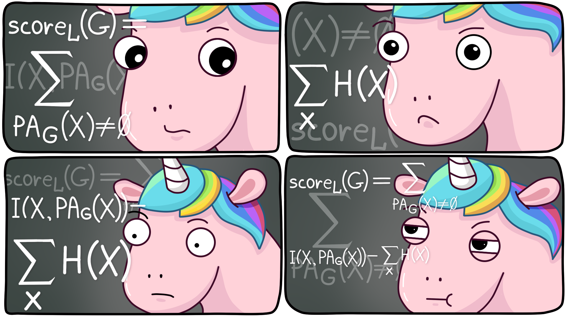
The first one is the graph likelihood estimate:

Here

P A_{G} (X)

$PA_G(X)$ - many vertex parents

X

$X$ ,

I (X, Y)

$I(X, Y)$ - joint information of quantities

X

$X$ and

Y

$Y$ , and

H (X)

$H(X)$ Is the entropy of the quantity

X

$X$ ... In fact, the second term does not depend on the structure of the graph, therefore, as a rule, only the first is considered. But you can see that the likelihood does not decrease with the addition of new edges - this must be taken into account when comparing.

It is important to understand that such an assessment only works for comparing Bayesian networks (output of the PC algorithm), because in real PAGs (output of FCI, FCI + algorithms), double edges have completely different semantics.

Therefore, I compared the orientation of the edges with my algorithm and the classic PC: The

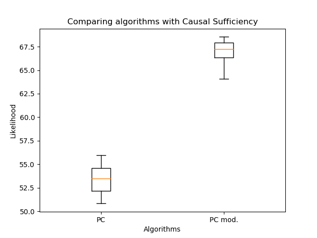
modified orientation of the edges allowed a significant increase in the likelihood compared to the classic algorithm. But now it's important to compare the number of edges:

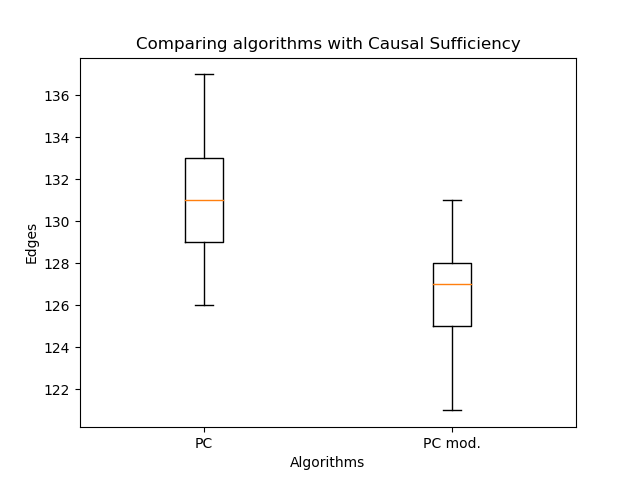
There are even fewer of them - this is expected. So even with fewer edges it is possible to recover a more plausible graph structure! Here you might argue that the likelihood does not decrease with the number of edges. The point is that the resulting graph in the general case is not a subgraph of the graph obtained by the classical PC-algorithm. Double edges may appear instead of single edges, and single edges may change direction. So no handicraft!

Comparing Models - 2: Using a Classification Approach

Let's move on to the second way of comparison. We will use the PC-algorithm to construct a causal graph and select a random acyclic graph from it. After that, we will generate the data at each vertex as a linear combination of the values at the parent vertices with the coefficients

\pm [0, 2, 0, 8]

$\pm[0,2, 0,8]$ with the addition of Gaussian noise. I took the idea for such a generation from the article "Towards Robust and Versatile Causal Discovery for Business Applications" (Borboudakis et al., 2016). The vertices that have no parents were generated from a normal distribution - with parameters as in the dataset for the corresponding vertex.

When the data is received, we apply the algorithms that we want to evaluate to it. Moreover, we already have a true causal graph. It remains only to understand how to compare the resulting graphs with the true one. In "Robust reconstruction of causal graphical models based on conditional 2-point and 3-point information" (Affeldt et al., 2015), it was suggested to use classification terminology. We will assume that the drawn edge is a Positive class, and the non-drawn one is Negative. Then True Positive (

T P

$TP$ ) Is when we have drawn the same edge as in the true causal graph, and False Positive (

F P

$FP$ ) - if an edge is drawn that is not in the true causal graph. We will evaluate these values from the point of view of the skeleton.

To take into account directions, we introduce

T P_{m i s o r i e n t}

$TP_{misorient}$ for edges that are displayed correctly, but with the wrong direction. After that, we will consider it like this:

$TP' = TP - TP_{misorient}$
$FP' = FP + TP_{misorient}$

Then you can read

F_{1}

$F_1$ -size both for the skeleton and taking into account the orientation (obviously, in this case, it will not be higher than that for the skeleton). However, in the case of the PC algorithm, a double edge adds to

T P_{m i s o r i e n t}

$TP_{misorient}$ only

0.5

$0.5$ , but not

1

$1$ , because one of the real edges is still deduced (without Causal Sufficiency, this would be wrong).

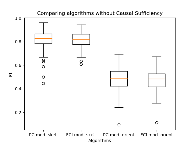
Finally, let's compare the algorithms:

The first two graphs are a comparison of the skeletons of the PC-algorithm: the classic one and with the new edge orientation. They are needed to show the upper border

F_{1}

$F_1$ -measures. The second two are comparing these algorithms with regard to orientation. As you can see, there is no win.

Compare Models - 3: Turn off Causal Sufficiency

Now let's "close" some variables in the true graph and in the synthetic data after generation. This will turn off Causal Sufficiency. But it will be necessary to compare the results not with the true graph, but with the one obtained as follows:

the edges from the parents of the hidden vertex will be drawn to its children,
connect all children of the hidden vertex with a double edge.

We will already compare the FCI + algorithms (with modified edge orientation and with the classical one):

And now, when Causal Sufficiency is not met, the result of the new orientation becomes much better.

Another important observation has appeared - the PC and FCI algorithms build almost identical skeletons in practice. Therefore, I compared their output with the orientation of the edges, which I proposed in my work.

It turned out that the algorithms practically do not differ in quality. In this case, PC is a step of the skeleton construction algorithm inside the FCI. Thus, using the orientation PC algorithm, as in the FCI algorithm, is a good solution to increase the speed of link inference.

Output

I will briefly summarize what we talked about in this article:

How the task of deriving causal links can arise in a large IT company.
What are spurious correlations and how they can interfere with Feature Selection.
What algorithms for inference links exist and are used most often.
What difficulties can arise when deriving causal graphs?
What is the comparison of causal graphs and how to deal with it.

If you are interested in the topic of causal inference, check out my other article - it has more theory. There I write in detail about the basic terms that are used in the inference of links, as well as how the classical algorithms work and the orientation of the edges that I proposed.

We analyze the causal relationships of VK metrics