1.1 What is Decision Tree?
1.1.1 Decision Tree Example
For example, we have the following dataset (date set): weather, temperature, humidity, wind, golf. Depending on the weather and everything else, we went (〇) or didn't (×) play golf. Let's assume that we have 14 preconceived options.
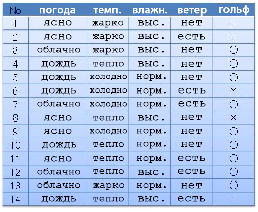
From this data, we can compose a data structure showing in which cases we went to golf. This structure is called the Decision Tree due to its branchy shape.
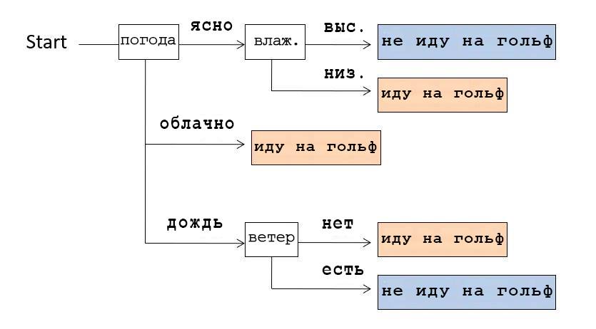
For example, if we look at the Decision Tree shown in the picture above, we realize that we checked the weather first. If it was clear, we checked the humidity: if it is high, then we did not go to play golf, if it is low, we went. And if the weather was cloudy, then they went to play golf, regardless of other conditions.
1.1.2 About this article
There are algorithms that create such Decision Trees automatically based on the available data. In this article, we will use the Python ID3 algorithm.
This article is the first in a series. The following articles:
(Note of the translator: “if you are interested in the sequel, please let us know in the comments.”)
- Fundamentals of Python Programming
- Essential library basics for Pandas data analysis
- Data structure basics (in the case of Decision Tree)
- Basics of information entropy
- Learning an algorithm for generating a Decision Tree
1.1.3 A little about Decision Tree
Decision Tree generation is related to supervised machine learning and classification. Classification in machine learning is a way to create a model leading to the correct answer based on training on the date set with the correct answers and data leading to them. Deep Learning, which has been very popular in recent years, especially in the field of image recognition, is also part of machine learning based on the classification method. The difference between Deep Learning and Decision Tree is whether the final result is reduced to a form in which a person understands the principles of generating the final data structure. The peculiarity of Deep Learning is that we get the final result, but do not understand the principle of its generation. Unlike Deep Learning, the Decision Tree is easy to understand by humans, which is also an important feature.
This feature of Decision Tree is good not only for machine learning, but also for date mining, where understanding of the data by the user is also important.
1.2 About the ID3 algorithm
ID3 is a Decision Tree generation algorithm developed in 1986 by Ross Quinlan. It has two important features:
- Categorical data. This is data similar to our example above (go golf or not), data with a specific categorical label. ID3 cannot use numeric data.
- Information entropy is an indicator that indicates a sequence of data with the least variance of the properties of a class of values.
1.2.1 About using numerical data
Algorithm C4.5, which is a more advanced version of ID3, can use numerical data, but since the basic idea is the same, in this series of articles, we will use ID3 first.
1.3 Development environment
The program that I described below, I tested and ran under the following conditions:
- Jupyter Notebooks (using Azure Notebooks)
- Python 3.6
- Libraries: math, pandas, functools (didn't use scikit-learn, tensorflow, etc.)
1.4 Sample program
1.4.1 Actually, the program
First, let's copy the program into Jupyter Notebook and run it.
import math
import pandas as pd
from functools import reduce

#
d = {
    "":["","","","","","","","","","","","","",""],
    "":["","","","","","","","","","","","","",""],
    "":["","","","","","","","","","","","","",""],
    "":["","","","","","","","","","","","","",""],
    #   -    ,  ,
    #    .
    "":["×","×","○","○","○","×","○","×","○","○","○","○","○","×"],
}
df0 = pd.DataFrame(d)

# -   ,  - pandas.Series,
#   -
#    s   value_counts()     ,
#       ,   ,  items().
#         ,   sorted,
#
#  ,  ,     :  (k)   (v).
cstr = lambda s:[k+":"+str(v) for k,v in sorted(s.value_counts().items())]

#   Decision Tree
tree = {
    # name:    ()
    "name":"decision tree "+df0.columns[-1]+" "+str(cstr(df0.iloc[:,-1])),
    # df: ,     ()
    "df":df0,
    # edges:   (),    ,
    #   ,     .
    "edges":[],
}

#  ,      ,   open
open = [tree]

# -   .
#  - pandas.Series、  -
entropy = lambda s:-reduce(lambda x,y:x+y,map(lambda x:(x/len(s))*math.log2(x/len(s)),s.value_counts()))

# ,  open
while(len(open)!=0):
    #    open  ,
    #   ,
    n = open.pop(0)
    df_n = n["df"]

    #  ,      0,
    #
    if 0==entropy(df_n.iloc[:,-1]):
        continue
    #  ,
    attrs = {}
    #   ,
    for attr in df_n.columns[:-1]:
        #  ,         ,
        #      ,  .
        attrs[attr] = {"entropy":0,"dfs":[],"values":[]}
        #      .
        #  , sorted      ,
        #       ,    .
        for value in sorted(set(df_n[attr])):
            #
            df_m = df_n.query(attr+"=='"+value+"'")
            #  ,
            attrs[attr]["entropy"] += entropy(df_m.iloc[:,-1])*df_m.shape[0]/df_n.shape[0]
            attrs[attr]["dfs"] += [df_m]
            attrs[attr]["values"] += [value]
            pass
        pass
    #      ,    ,
    #    .
    if len(attrs)==0:
        continue
    #
    attr = min(attrs,key=lambda x:attrs[x]["entropy"])
    #
    #  ,   ,      open.
    for d,v in zip(attrs[attr]["dfs"],attrs[attr]["values"]):
        m = {"name":attr+"="+v,"edges":[],"df":d.drop(columns=attr)}
        n["edges"].append(m)
        open.append(m)
    pass

#
print(df0,"\n-------------")
#     ,  - tree:  ,
# indent:    indent,
#   -   .
#            .
def tstr(tree,indent=""):
    #     .
    #       (      0),
    #      df,   ,   .
    s = indent+tree["name"]+str(cstr(tree["df"].iloc[:,-1]) if len(tree["edges"])==0 else "")+"\n"
    #     .
    for e in tree["edges"]:
        #          .
        #      indent  .
        s += tstr(e,indent+"  ")
        pass
    return s
#      .
print(tstr(tree))
1.4.2 Result
If you run the above program, our Decision Tree will be represented as a symbol table as shown below.
decision tree  ['×:5', '○:9']
  =
    =['○:2']
    =['×:3']
  =['○:4']
  =
    =['×:2']
    =['○:3']
1.4.3 Change the attributes (data arrays) that we want to explore
The last array in the date set d is a class attribute (the array of data we want to classify).
d = {
"":["","","","","","","","","","","","","",""],
"":["","","","","","","","","","","","","",""],
"":["","","","","","","","","","","","","",""],
"":["×","×","○","○","○","×","○","×","○","○","○","○","○","×"],}
#   -    ,  ,    .
"":["","","","","","","","","","","","","",""],
}
For example, if you swap the arrays "Golf" and "Wind", as shown in the example above, you get the following result:
decision tree  [':6', ':8']
  =×
    =
      =
        =[':1', ':1']
      =[':1']
    =[':2']
  =○
    =
      =[':1']
      =[':1']
    =
      =[':2']
      =[':1']
      =[':1']
    =[':3']
In essence, we create a rule in which we tell the program to branch out first by the presence and absence of wind and by whether we are going to play golf or not.
Thanks for reading!
We will be very happy if you tell us if you liked this article, was the translation clear, was it useful to you?