It is convenient to process text in natural language using Python, since it is a fairly high-level programming tool, has a well-developed infrastructure, and has proven itself in the field of data analysis and machine learning. Several libraries and frameworks have been developed by the community for solving NLP problems in Python. In our work, we will use an interactive web tool for developing python scripts Jupyter Notebook, the NLTK library for text analysis and the wordcloud library for building a word cloud.
The network contains a fairly large amount of material on the topic of text analysis, but in many articles (including Russian-language ones) it is proposed to analyze the text in English. The analysis of the Russian text has some specifics of using the NLP toolkit. As an example, consider the frequency analysis of the text of the story "Snowstorm" by A. Pushkin.
Frequency analysis can be roughly divided into several stages:
- Loading and browsing data
- Text cleaning and preprocessing
- Remove stop words
- Translating words into basic form
- Calculating the statistics of the occurrence of words in the text
- Cloud visualization of word popularity
The script is available at github.com/Metafiz/nlp-course-20/blob/master/frequency-analisys-of-text.ipynb , source - github.com/Metafiz/nlp-course-20/blob/master/pushkin -metel.txt
Loading data
We open the file using the open built-in function, specify the reading mode and encoding. We read the entire contents of the file, as a result we get the string text:
f = open('pushkin-metel.txt', "r", encoding="utf-8")
text = f.read()
The length of the text - the number of characters - can be obtained with the standard len function:
len(text)
A string in python can be represented as a list of characters, so index access and slicing operations are also possible for working with strings. For example, to view the first 300 characters of text, just run the command:
text[:300]
Pre-processing (preprocessing) of text
To carry out frequency analysis and determine the subject of the text, it is recommended to clear the text from punctuation marks, extra whitespace characters and numbers. You can do this in a variety of ways - using built-in string functions, using regular expressions, using list processing, or in another way.
First, let's convert characters to a single case, for example, lower:
text = text.lower()
We use the standard punctuation character set from the string module:
import string
print(string.punctuation)
string.punctuation is a string. The set of special characters to be removed from the text can be expanded. It is necessary to analyze the source text and identify the characters that should be removed. Let's add line breaks, tabs and other symbols that are found in our source text to punctuation marks (for example, the character with the code \ xa0):
spec_chars = string.punctuation + '\n\xa0«»\t—…'
To remove characters, we use element-wise processing of the string - divide the original text string into characters, leave only characters that are not in the spec_chars set, and again combine the list of characters into a string:
text = "".join([ch for ch in text if ch not in spec_chars])
You can declare a simple function that removes the specified character set from the source text:
def remove_chars_from_text(text, chars):
    return "".join([ch for ch in text if ch not in chars])
It can be used both to remove special characters and to remove numbers from the original text:
text = remove_chars_from_text(text, spec_chars)
text = remove_chars_from_text(text, string.digits)
Tokenizing text
For further processing, the cleared text must be split into its component parts - tokens. Natural language text analysis uses symbol, word, and sentence breakdowns. The partitioning process is called tokenization. For our task of frequency analysis, it is necessary to break the text into words. To do this, you can use the ready-made method of the NLTK library:
from nltk import word_tokenize
text_tokens = word_tokenize(text)
The variable text_tokens is a list of words (tokens). To calculate the number of words in the preprocessed text, you can get the length of the token list:
len(text_tokens)
To display the first 10 words, let's use the slice operation:
text_tokens[:10]
To use the frequency analysis tools of the NLTK library, you need to convert the list of tokens to the Text class, which is included in this library:
import nltk
text = nltk.Text(text_tokens)
Let's deduce the type of the variable text:
print(type(text))
Slice operations are also applicable to a variable of this type. For example, this action will output the first 10 tokens from the text:
text[:10]
Calculating the statistics of the occurrence of words in the text
The FreqDist (frequency distributions) class is used to calculate the statistics of word frequency distribution in the text:
from nltk.probability import FreqDist
fdist = FreqDist(text)
Trying to display the fdist variable will display a dictionary containing tokens and their frequencies - the number of times these words appear in the text:
FreqDist({'': 146, '': 101, '': 69, '': 54, '': 44, '': 42, '': 39, '': 39, '': 31, '': 27, ...})
You can also use the most_common method to get a list of tuples with the most common tokens:
fdist.most_common(5)

[('', 146), ('', 101), ('', 69), ('', 54), ('', 44)]
The frequency of distribution of words in a text can be visualized using a graph. The FreqDist class contains a built-in plot method for plotting such a plot. It is necessary to indicate the number of tokens, the frequencies of which will be shown on the chart. With the parameter cumulative = False, the graph illustrates Zipf's law : if all words of a long enough text are ordered in descending order of frequency of their use, then the frequency of the nth word in such a list will be approximately inversely proportional to its ordinal number n.
fdist.plot(30,cumulative=False)
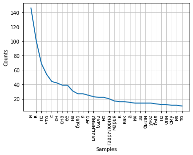
It can be noted that at the moment the highest frequencies have conjunctions, prepositions and other service parts of speech that do not carry a semantic load, but only express semantic-syntactic relations between words. In order for the results of the frequency analysis to reflect the subject of the text, it is necessary to remove these words from the text.
Remove stop words
Stop words (or noise words), as a rule, include prepositions, conjunctions, interjections, particles and other parts of speech that are often found in the text, are service ones and do not carry a semantic load - they are redundant.
The NLTK library contains ready-made stop-word lists for various languages. Let's get a list of one hundred words for the Russian language:
from nltk.corpus import stopwords
russian_stopwords = stopwords.words("russian")
It should be noted that stop words are context sensitive - for texts of different topics, stop words may differ. As in the case with special characters, it is necessary to analyze the source text and identify stop words that are not included in the standard set.
The stopword list can be extended using the standard extend method:
russian_stopwords.extend(['', ''])
After removing the stop words, the distribution frequency of tokens in the text is as follows:
fdist_sw.most_common(10)

[('', 23),
 ('', 20),
 ('', 17),
 ('', 9),
 ('', 9),
 ('', 8),
 ('', 7),
 ('', 6),
 ('', 6),
 ('', 6)]
As you can see, the results of frequency analysis have become more informative and more accurately reflect the main topic of the text. However, we see in the results such tokens as "vladimir" and "vladimira", which are, in fact, one word, but in different forms. To correct this situation, it is necessary to bring the words of the source text to their bases or their original form - to carry out stemming or lemmatization.
Cloud visualization of word popularity
At the end of our work, we visualize the results of the frequency analysis of the text in the form of a "word cloud".
For this we need the wordcloud and matplotlib libraries:
from wordcloud import WordCloud
import matplotlib.pyplot as plt
%matplotlib inline
To build a word cloud, a string must be passed to the method as input. To convert the list of tokens after preprocessing and removing stop words, we will use the join method, specifying a space as a separator:
text_raw = " ".join(text)
Let's call the method for constructing the cloud:
wordcloud = WordCloud().generate(text_raw)
As a result, we get such a "word cloud" for our text:
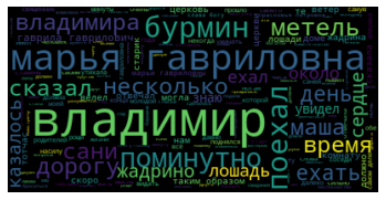
Looking at it, you can get a general idea of the subject matter and the main characters of the work.