
Can a query running in parallel use less CPU and run faster than a query running sequentially?
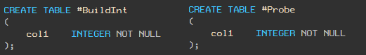
Yes! For demonstration, I will use two tables with one column type
integer.
Note - TSQL script in the form of text is at the end of the article.
Generating demo data
We
#BuildIntinsert 5,000 random integers into the table (so that you have the same values as mine, I use RAND with seed and a WHILE loop). Insert 5,000,000 records into the

table
#Probe.

Sequential plan
Now let's write a query to count the number of matches of values in these tables. We use the MAXDOP 1 hint to make sure that the query will not be executed in parallel.
Its execution plan and statistics are as follows:

This query takes 891ms and uses 890ms of CPU.
Parallel plan
Now let's run the same query with MAXDOP 2. The

query takes 221 ms and uses 436 ms of CPU. The execution time has decreased four times, and the CPU usage has halved!
Magic Bitmap
The reason why parallel query execution is much more efficient is because of the Bitmap operator.
Let's take a close look at the actual execution plan for the parallel query:

And compare it with the sequential plan:

The principle of the Bitmap operator is well documented, so here I will only provide a brief description with links to the documentation at the end of the article.
Hash Join
Hash join is done in two steps:
- The stage of "building" (English - build). All rows of one of the tables are read and a hash table is created for the join keys.
- The stage of "verification" (English - probe). All rows of the second table are read, the hash is calculated by the same hash function using the same connection keys, and a matching bucket is found in the hash table.
Naturally, due to possible hash collisions, it is still necessary to compare the real values of the keys.
Translator's note: for more details on how hash join works, see the article Visualizing and Dealing with Hash Match Join
Bitmap in sequential plans
Many people don't know that Hash Match, even in sequential requests, always uses a bitmap. But in this way, you will not see it explicitly, because it is part of the internal implementation of the Hash Match operator.
HASH JOIN at the stage of building and creating a hash table sets one (or more) bits in the bitmap. You can then use the bitmap to efficiently match the hash values without the overhead of accessing the hash table.
With a sequential plan, a hash is calculated for each row of the second table and checked against a bitmap. If the corresponding bits in the bitmap are set, then there can be a match in the hash table, so the hash table is checked next. Conversely, if none of the bits corresponding to the hash value are set, then we can be sure that there are no matches in the hash table, and we can immediately discard the checked string.
The relatively low cost of building a bitmap is offset by the time savings in not checking strings for which there is definitely no match in the hash table. This optimization is often effective because checking the bitmap is much faster than checking the hash table.
Bitmap in parallel plans
In a parallel plan, the bitmap is displayed as a separate Bitmap statement.
When moving from the construction stage to the verification stage, the bitmap is passed to the HASH MATCH operator from the side of the second (probe) table. At a minimum, the bitmap is passed to the probe side before the JOIN and the exchange operator (Parallelism).
Here, the bitmap can exclude strings that do not satisfy the join condition before they are passed to the exchange statement.
Of course, there are no exchange statements in sequential plans, so moving the bitmap outside of the HASH JOIN does not provide any additional advantage over the "embedded" bitmap inside the HASH MATCH statement.
In some situations (albeit only in a parallel plan), the optimizer may move the Bitmap further down the plane on the probe side of the connection.
The idea here is that the sooner the rows are filtered, the less overhead will be required to move data between statements, and it might even be possible to eliminate some operations.
Also, the optimizer usually tries to place simple filters as close to the leaves as possible: it is most efficient to filter rows as early as possible. However, I must mention that the bitmap we are talking about is added after the optimization is complete.
The decision to add this (static) type of bitmap to the plan after optimization is made based on the expected selectivity of the filter (so accurate statistics are important).
Moving a bitmap filter
Let's get back to the concept of moving the bitmap filter to the probe side of the connection.
In many cases, the bitmap filter can be moved to a Scan or Seek statement. When this happens, the plan predicate looks like this:

It applies to all rows that match the seek predicate (for Index Seek) or all rows for Index Scan or Table Scan. For example, the screenshot above shows a bitmap filter applied to the Table Scan for a heap table.
Going deeper ...
If a bitmap filter is built on a single integer or bigint column or expression, and is applied to a single integer or bigint column, then the Bitmap operator can be moved even further down the road, even further than the Seek or Scan operators.
The predicate will still appear in the Scan or Seek statements as in the example above, but now it will be marked with the INROW attribute, which means the filter is moved to the Storage Engine and applied to rows as they are read.
With this optimization, rows are filtered before the Query Processor sees the row. Only those strings that match the HASH MATCH JOIN are sent from the Storage Engine.
The conditions under which this optimization is applied depends on the version of SQL Server. For example, in SQL Server 2005, in addition to the conditions stated earlier, the probe column must be defined as NOT NULL. This limitation has been relaxed in SQL Server 2008.
You may be wondering how INROW optimizations affect performance. Will moving the operator as close to Seek or Scan as possible be as efficient as filtering in the Storage Engine? I will answer this interesting question in other articles. And here we will also look at MERGE JOIN and NESTED LOOP JOIN.
Other JOIN options
Using nested loops without indices is a bad idea. We have to completely scan one of the tables for every row from the other table - a total of 5 billion comparisons. This request is likely to take a very long time.
Merge Join
This type of physical join requires sorted input, so a forced MERGE JOIN causes a sort to be present before it. The sequential plan looks like this:
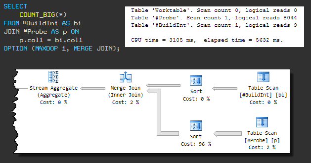
The query now uses 3105ms of CPU, and the total execution time is 5632ms .
The increase in overall execution time is due to the fact that one of the sort operations is using tempdb (even though SQL Server has sufficient memory for the sort).
The leak into tempdb occurs because the default memory grant algorithm does not pre-reserve enough memory. Until we pay attention to this, it is clear that the request will not complete in less than 3105 ms.
Let's continue to force the MERGE JOIN, but allow parallelism (MAXDOP 2):

As in the parallel HASH JOIN we saw earlier, the bitmap filter is located on the other side of the MERGE JOIN closer to the Table Scan and is applied using INROW optimization.
With 468 ms CPU and 240 ms elapsed time, a MERGE JOIN with additional sorts is almost as fast as a parallel HASH JOIN ( 436 ms / 221 ms ).
But the parallel MERGE JOIN has one drawback: it reserves 330 KB of memory based on the expected number of rows to sort. Since these types of bitmaps are used after cost optimization, there is no adjustment to the estimate, even though only 2488 rows go through the bottom sort.
A Bitmap statement can appear in a plan with a MERGE JOIN only with a subsequent blocking statement (for example, Sort). The blocking operator must receive all required values as input before it generates the first line to output. This ensures that the bitmap is completely full before rows from the JOIN table are read and checked against it.
It is not necessary for the blocking statement to be on the other side of the MERGE JOIN, but it is important which side the bitmap is used on.
With indices
If suitable indices are available, the situation is different. The distribution of our "random" data is such that
#BuildInta unique index can be created on the table . And the table #Probecontains duplicates, so you have to get by with a non-unique index:

This change will not affect the HASH JOIN (both in serial and parallel). HASH JOIN cannot use indexes, so plans and performance remain the same.
Merge Join
MERGE JOIN no longer needs to perform a many-to-many join operation and no longer requires a Sort operator on the input.
The absence of a blocking sort operator means that Bitmap cannot be used.
As a result, we see a sequential plan, regardless of the MAXDOP parameter, and the performance is worse than the parallel plan before the indexes were added: 702 ms CPU and 704 ms elapsed time:

However, there is a noticeable improvement over the original sequential MERGE JOIN plan ( 3105 ms / 5632 ms ). This is due to the elimination of sorting and better one-to-many join performance.
Nested Loops Join
As you might expect, NESTED LOOP performs significantly better. Similar to the MERGE JOIN, the optimizer decides not to use concurrency:

This is the most efficient plan so far - only 16ms CPU and 16ms spent time.
Of course, this assumes that the data needed to complete the request is already in memory. Otherwise, each lookup in the probe table will generate random I / O.
On my laptop performance of NESTED LOOP cold cache took 78 ms CPU and 2152 ms, elapsed time. Under the same circumstances, MERGE JOIN used 686 ms CPU and 1471 ms . HASH JOIN - 391 ms CPU and905 ms .
MERGE JOIN and HASH JOIN benefit from large, possibly sequential I / O using read-ahead.
Additional Resources
Parallel Hash Join (Craig Freedman)
Query Execution Bitmap Filters (SQL Server Query Processing Team)
Bitmaps in Microsoft SQL Server 2000 (MSDN article)
Interpreting Execution Plans Containing Bitmap Filters (SQL Server Documentation)
Understanding Hash Joins (SQL Server Documentation)
Test script
USE tempdb;
GO
CREATE TABLE #BuildInt
(
    col1    INTEGER NOT NULL
);
GO
CREATE TABLE #Probe
(
    col1    INTEGER NOT NULL
);
GO

-- Load 5,000 rows into the build table
SET NOCOUNT ON;
SET STATISTICS XML OFF;

DECLARE @I INTEGER = 1;

INSERT #BuildInt
    (col1)
VALUES
    (CONVERT(INTEGER, RAND(1) * 2147483647));

WHILE @I < 5000
BEGIN
    INSERT #BuildInt
        (col1)
    VALUES
        (RAND() * 2147483647);
    SET @I += 1;
END;

-- Load 5,000,000 rows into the probe table
SET NOCOUNT ON;
SET STATISTICS XML OFF;

DECLARE @I INTEGER = 1;

INSERT #Probe
    (col1)
VALUES
    (CONVERT(INTEGER, RAND(2) * 2147483647));

BEGIN TRANSACTION;
WHILE @I < 5000000
BEGIN
    INSERT #Probe
        (col1)
    VALUES
        (CONVERT(INTEGER, RAND() * 2147483647));

    SET @I += 1;

    IF @I % 25 = 0
    BEGIN
        COMMIT TRANSACTION;
        BEGIN TRANSACTION;
    END;
END;

COMMIT TRANSACTION;
GO
-- Demos
SET STATISTICS XML OFF;
SET STATISTICS IO, TIME ON;

-- Serial
SELECT
    COUNT_BIG(*)
FROM #BuildInt AS bi
JOIN #Probe AS p ON
    p.col1 = bi.col1
OPTION (MAXDOP 1);

-- Parallel
SELECT
    COUNT_BIG(*)
FROM #BuildInt AS bi
JOIN #Probe AS p ON
    p.col1 = bi.col1
OPTION (MAXDOP 2);

SET STATISTICS IO, TIME OFF;

-- Indexes
CREATE UNIQUE CLUSTERED INDEX cuq ON #BuildInt (col1);
CREATE CLUSTERED INDEX cx ON #Probe (col1);

-- Vary the query hints to explore plan shapes

SELECT
    COUNT_BIG(*)
FROM #BuildInt AS bi
JOIN #Probe AS p ON
    p.col1 = bi.col1
OPTION (MAXDOP 1, MERGE JOIN);
GO
DROP TABLE #BuildInt, #Probe;
Read more:
- Errors when working with date and time in SQL Server
- Window functions with a "window" or how to use a frame