Machine learning. Neural networks (part 1): The process of training the perceptron
In this article, we will use a neural network to model the execution of logical OR operations; XOR, which is a kind of "Hello World" application for neural networks.
The article will step by step describe the process of such modeling using TensorFlow.js.
So let's build a neural network for the logical OR operation. At the input, we will always give two signals X 1 and X 2 , and at the output we will receive one output signal Y. To train the neural network, we also need a training dataset (Figure 1).

Figure 1 - A training dataset and a model for modeling a logical OR operation
To understand what structure of a neural network to set, let's imagine a training dataset on a coordinate plane with axes X 1 and X 2 (Figure 2, left).
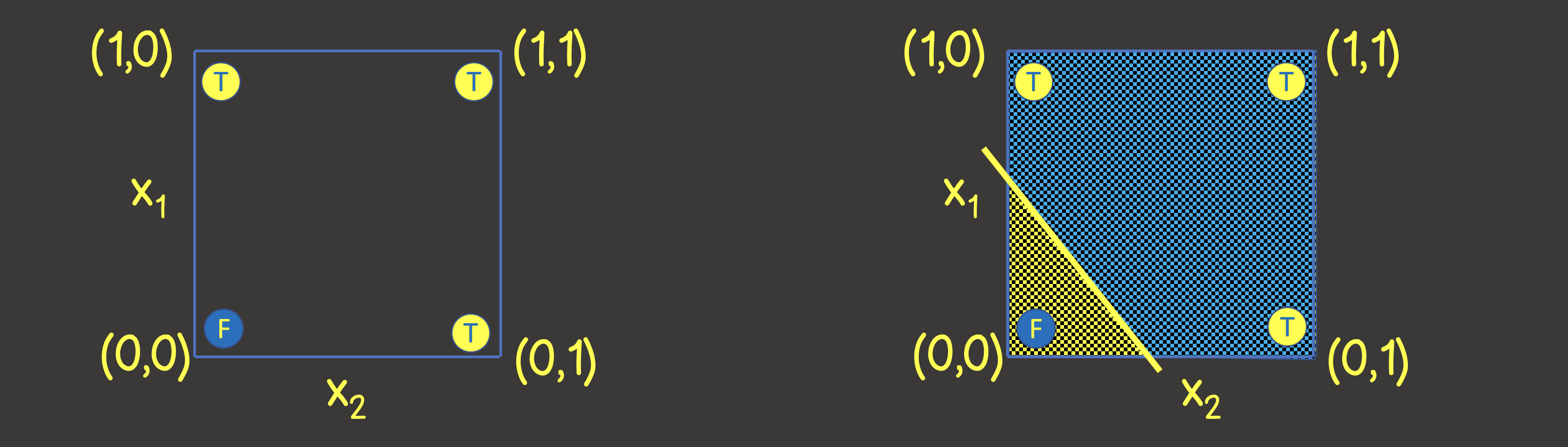
Figure 2 - Training set on the coordinate plane for logical OR operation
Please note that to solve this problem, it is enough for us to draw a line that would divide the plane in such a way that on one side of the line there are all TRUE values, and on the other - all FALSE values (Figure 2, right). We also know that one neuron in a neural network (perceptron) can perfectly cope with this purpose, the output value of which is calculated from the input signals as:
which is a mathematical representation of the equation of a straight line.
In view of the fact that our values are in the range from 0 to 1, we also apply the sigmoid activation function. Thus, our neural network looks like in Figure 3.

Figure 3 - A neural network for training logical OR operation
So let's solve this problem using TensorFlow.js.
First, we need to convert the training dataset to tensors. A tensor is a container of data that can haveaxes and an arbitrary number of elements along each of the axes. Most with tensors are familiar with mathematics - vectors (tensor with one axis), matrices (tensor with two axes - rows, columns).
To define the training dataset, the first axis (axis 0) is always the axis along which all available data sample instances are located (Figure 4).
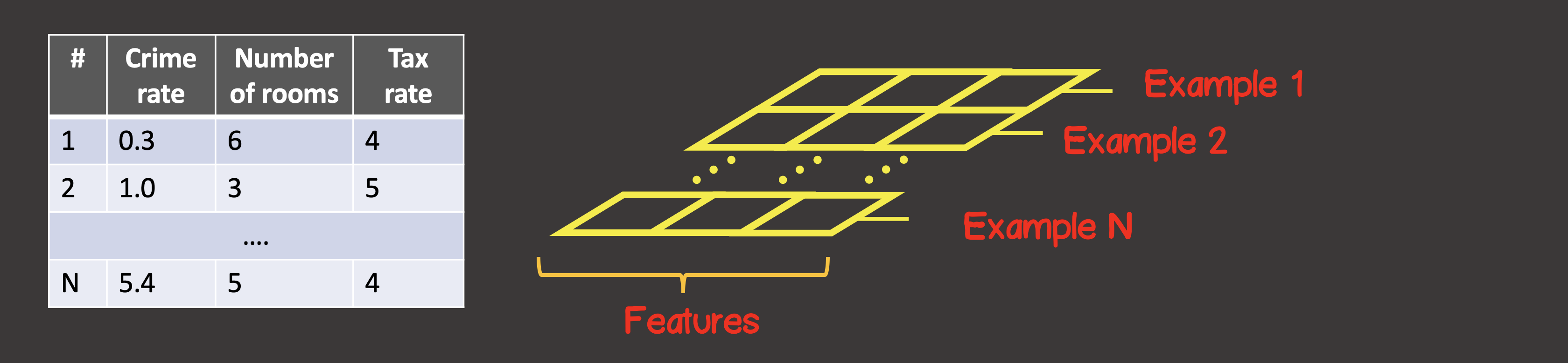
Figure 4 - Tensor structure
In our specific case, we have 4 instances of data samples (Figure 1), which means that the input tensor along the first axis will have 4 elements. Each element of the training sample is a vector consisting of two elements X 1 , X 2 . Thus, the input tensor has 2 axes (matrix), along the first axis there are 4 elements, along the second axis - 2 elements.
const input = [[0, 0], [1, 0], [0, 1], [1, 1]];
const inputTensor = tf.tensor(input, [input.length, 2]);
Likewise, convert the output to a tensor. As for the input signals, along the first axis we have 4 elements, and each element contains a vector containing one value:
const output = [[0], [1], [1], [1]]
const outputTensor = tf.tensor(output, [output.length, 1]);
Let's create a model using the TensorFlow API:
const model = tf.sequential();
model.add(
      tf.layers.dense({ inputShape: [2], units: 1, activation: 'sigmoid' })
);
Model creation will always start with a call to tf.sequential () . The main building block of a model is layers. We can connect to the model as many layers in the neural network as we need. Here we use a dense layer, which means that every neuron in the next layer has a connection with every neuron in the previous layer. For example, if we have two dense layers, in the first layer neurons, and in the second - , then the total number of connections between layers will be ...
In our case, as we can see, the neural network consists of one layer, in which there is one neuron, therefore units are set to one.
Also, for the first layer of the neural network, we must set the inputShape , since each input instance is represented by a vector of two values X 1 and X 2 , therefore inputShape = [2] . Note that there is no need to set inputShape for intermediate layers - TensorFlow can determine this value from the units value of the previous layer.
Also, if necessary, each layer can be assigned an activation function, we determined above that this will be a sigmoid function. The currently available activation functions in TensorFlow can be found here .
Next, we need to compile the model (see API here ), while we need to set two required parameters - this is the error function and the kind of optimizer that will look for its minimum:
model.compile({
    optimizer: tf.train.sgd(0.1),
    loss: 'meanSquaredError'
});
We set a stochastic gradient descent with a training step of 0.1 as the optimizer.
The list of implemented optimizers in the library: tf.train.sgd , tf.train.momentum , tf.train.adagrad , tf.train.adadelta , tf.train.adam , tf.train.adamax , tf.train.rmsprop .
In practice, by default, you can immediately choose the adam optimizer, which has the best model convergence rates, in contrast to sgd - the learning rate at each stage of training is set depending on the history of previous steps and is not constant throughout the entire learning process.
As an error function, it is given by the root mean square error function:
The model is set, and the next step is the process of training the model, for this the fit method must be called on the model :
async function initModel() {
    // skip for brevity

    await model.fit(trainingInputTensor, trainingOutputTensor, {
        epochs: 1000,
        shuffle: true,
        callbacks: {
            onEpochEnd: async (epoch, { loss }) => {
                // any actions on during any epoch of training
                await tf.nextFrame();
            }
        }
    })
}
We have set that the learning process should consist of 100 learning steps (number of learning epochs); also at each next epoch - the input data should be shuffled in random order ( shuffle = true ) - which will speed up the process of model convergence, since there are few instances in our training dataset (4).
After the completion of the training process, we can use the predict method, which will calculate the output value based on new input signals.
const testInput = generateInputs(10);
const testInputTensor = tf.tensor(testInput, [testInput.length, 2]);

const output = model.predict(testInputTensor).arraySync();
The generateInputs method simply generates a 10x10 sample dataset that divides the coordinate plane into 100 squares:
The complete code is given here
import React, { useEffect, useState } from 'react';
import LossPlot from './components/LossPlot';
import Canvas from './components/Canvas';
import * as tf from "@tensorflow/tfjs";

let model;

export default () => {
    const [data, changeData] = useState([]);
    const [lossHistory, changeLossHistory] = useState([]);

    useEffect(() => {
        async function initModel() {
            const input = [[0, 0], [1, 0], [0, 1], [1, 1]];
            const inputTensor = tf.tensor(input, [input.length, 2]);

            const output = [[0], [1], [1], [1]]
            const outputTensor = tf.tensor(output, [output.length, 1]);

            const testInput = generateInputs(10);
            const testInputTensor = tf.tensor(testInput, [testInput.length, 2]);

            model = tf.sequential();
            model.add(
            tf.layers.dense({ inputShape:[2], units:1, activation: 'sigmoid'})
            );
            model.compile({
                optimizer: tf.train.adam(0.1),
                loss: 'meanSquaredError'
            });

            await model.fit(inputTensor, outputTensor, {
                epochs: 100,
                shuffle: true,
                callbacks: {
                    onEpochEnd: async (epoch, { loss }) => {
                        changeLossHistory((prevHistory) => [...prevHistory, {
                            epoch,
                            loss
                        }]);

                        const output = model.predict(testInputTensor)
                                                       .arraySync();
                        changeData(() => output.map(([out], i) => ({
                            out,
                            x1: testInput[i][0],
                            x2: testInput[i][1]
                        })));
                        await tf.nextFrame();
                    }
                }
            })
        }
        initModel();
    }, []);

    return (
        <div>
            <Canvas data={data} squareAmount={10}/>
            <LossPlot loss={lossHistory}/>
        </div>
    );
}

function generateInputs(squareAmount) {
    const step = 1 / squareAmount;
    const input = [];
    for (let i = 0; i < 1; i += step) {
        for (let j = 0; j < 1; j += step) {
            input.push([i, j]);
        }
    }
    return input;
}
In the following figure you will see part of the learning process:

Planker implementation:
Simulation of the logical operation XOR The
training set for this function is shown in Figure 6, and we will also place these points as we did for the logical operation OR on the coordinate plane
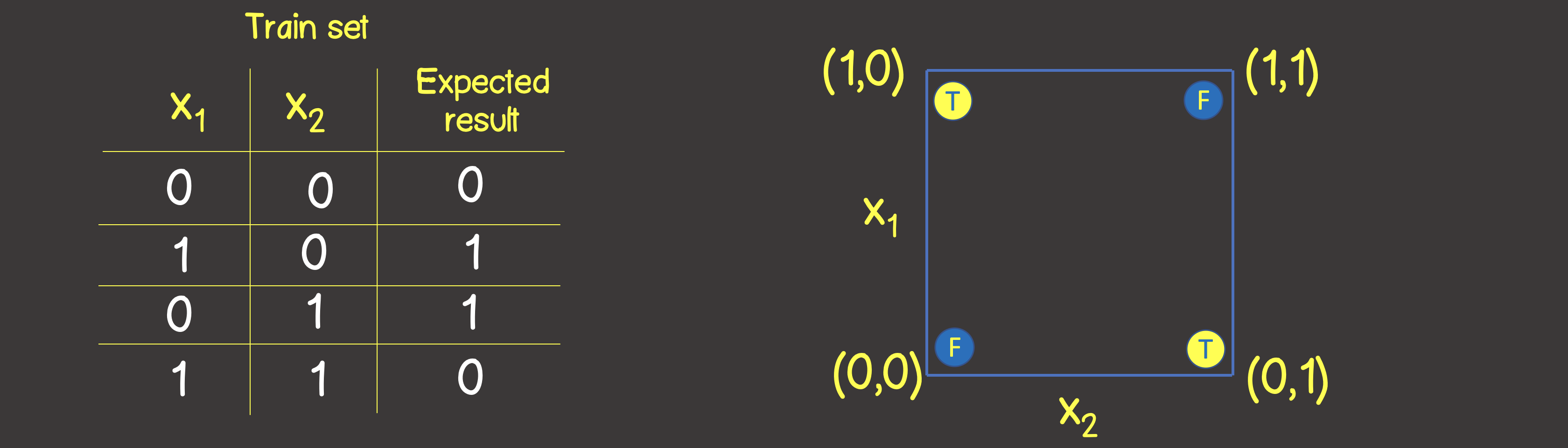
Figure 6 - Training dataset and model for modeling the logical operation EXCLUSIVE OR (XOR)
Please note that unlike the logical OR operation - you cannot divide the plane with one straight line, so that on one side there are all TRUE values, and on the other side - all FALSE . However, we can do this using two curves (Figure 7).
Obviously, in this case, one neuron in a layer is not enough - you need at least one more layer with two neurons, each of which would define one of the two lines on the plane.
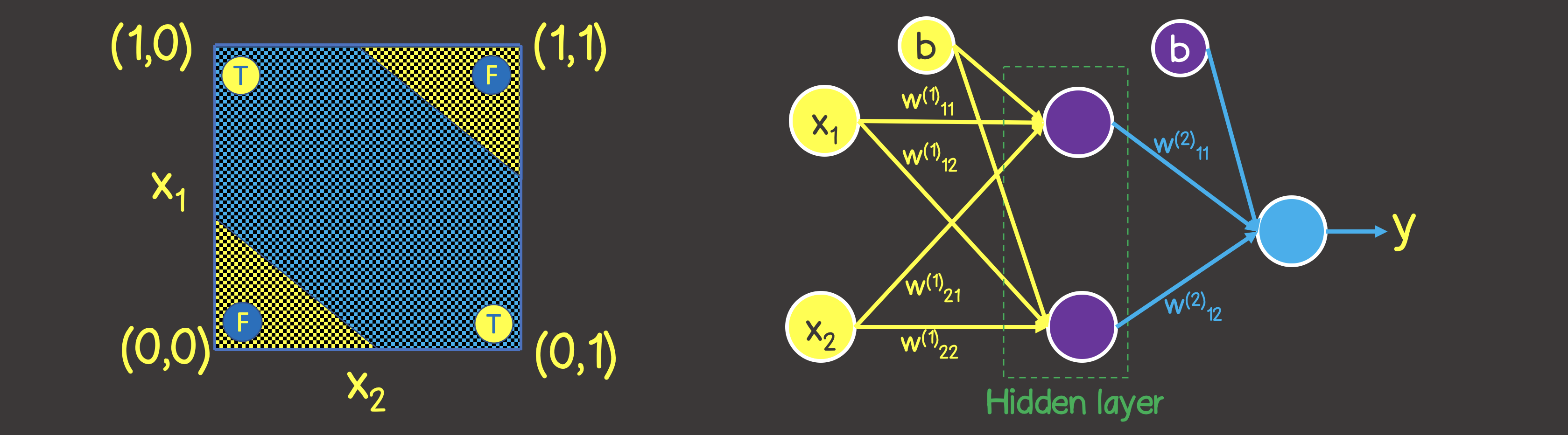
Figure 7 - Neural network model for the logical operation EXCLUSIVE OR (XOR)
In the previous code, we need to make changes in several places, one of which is the training dataset itself:
const input = [[0, 0], [1, 0], [0, 1], [1, 1]];
const inputTensor = tf.tensor(input, [input.length, 2]);

const output = [[0], [1], [1], [0]]
const outputTensor = tf.tensor(output, [output.length, 1]);
The second place is the changed structure of the model, according to Figure 7:
model = tf.sequential();
model.add(
    tf.layers.dense({ inputShape: [2], units: 2, activation: 'sigmoid' })
);
model.add(
    tf.layers.dense({ units: 1, activation: 'sigmoid' })
);
The learning process in this case looks like this:

Planker implementation:
Topic of the next article
In the next article we will describe how to solve problems related to the classification of objects into categories, based on a list of some features.