Render a RAW image

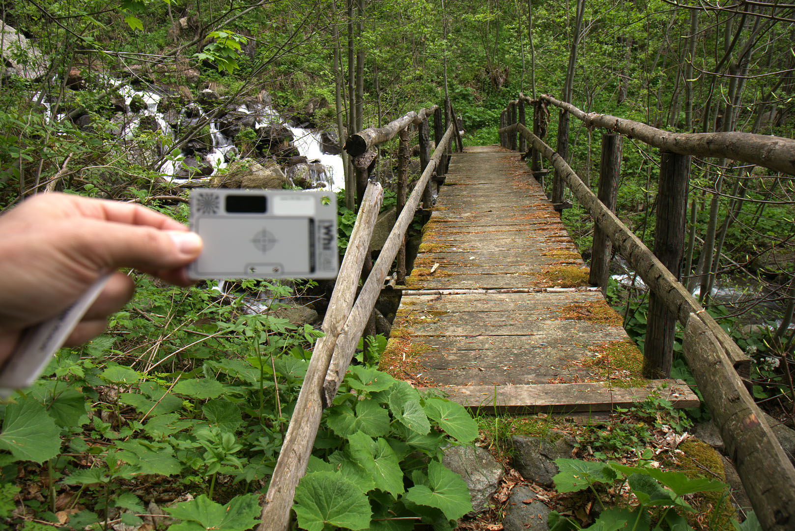
Figure: Photo 1: Nikon D610 photo with AF-S 24-120mm f / 4 lens at 24mm f / 8 ISO100



What are the basic steps for rendering a RAW image at a low level? In this article, I'll describe what's going on under the hood of digital camera converters, where raw data is converted into a viewable RAW image — sometimes called rendering. To demonstrate the transformation of information from the image at each step, I will use the photo shown at the beginning of the article, taken on a Nikon D610 with an AF-S 24-120mm f / 4 lens and 24mm f / 8 ISO100 settings.

Rendering is RAW conversion and editing

Rendering can be divided into two main processes: RAW conversion and editing. RAW conversion is necessary to turn the raw image data into a standard format that image editing, viewing programs and devices can understand. Typically, this is done using a RGB colorimetric color space such as Adobe or sRGB.



Editors take information about an image in a standard color space and apply adjustments to it to make the image more "fit" or "enjoyable" for the photographer.



An example of a clean RAW converter is dcraw by David Coffin. An example of a clean editor is Photoshop from Adobe. Most RAW converters actually combine RAW conversion functions with editor functions (eg Capture NX, LR, C1).

7 steps to basic RAW conversion

The boundary of where converting ends and editing starts is rather blurry, but depending on how you separate them, there are only 7 steps in the main process of converting a RAW file to a standard colorimetric color space - for example, sRGB. The steps do not have to go in that order, but the following sequence is pretty logical.

1. Load linear data from RAW file and subtract black levels.
2. Balance white.
3. Correct linear brightness.
4. Crop image data.
5. Restore original image from mosaic ( debayering ).
6. Apply color transformations and corrections.
7. Apply gamma.

In basic RAW conversion, the process remains linear until the very end. Ideally, the gamma curve in the last step is corrected by the device that displays the image, so the image processing system from the beginning to the end - from the moment when light hits the sensor to the moment when the light reaches the eye - is approximately linear. If you need to "honestly" render an image the way it got to the sensor, then this is all you need from a RAW converter.

+ Tone Mapping: Adapt to the dynamic range of the output device

However, as we will see, basic conversion of RAW files in existing digital cameras almost never gives a satisfactory result, since most of the output devices (photo paper, monitors) have inferior contrast ratios to what good digital cameras can capture. Therefore, it is practically necessary to perform tone correction to bring the wide dynamic range of the camera to the narrow dynamic range of the device. It can be a simple contrast curve - or a more complex tone mapping along with local and global adjustments for shadows, highlights, clarity, etc. (standard sliders in commercial editors and converter software). This is usually done when editing a render - but if you are aiming for "accurate" color,Ideally, the tone mapping should be part of the 6th step of color grading during RAW conversion (see.a great site by Alex Torgera describing color profiles).



After seven basic conversion steps, you can go to the editor in order to objectively correct imperfections identified in a particular frame and in a particular image output to the output device - and also make the image subjectively more pleasing to the artist's eye. For example, fix lens distortion and lateral chromatic aberration; apply noise reduction; apply a sharpening filter. It may be better to perform some of these functions in linear space before certain RAW conversion steps, but they are usually optional and can be done the same way in the editor after rendering in gamma space.



In this article, we'll focus on the basic rendering part of RAW conversion, leaving the tone mapping and editing for another time.

1. Load linear data from RAW file and subtract black levels

The first step in converting RAW is simply loading data from the RAW file into memory. Since RAW formats differ from camera to camera, most converters use variations of the open source LibRaw / dcraw programs. The following commands for LibRaw or dcraw will repackage the RAW into a linear 16-bit TIF that can be read by processing applications (Matlab, ImageJ, PS, etc.). There is no need to install the program, you just need the executable file to be in the PATH variable or to be in the same directory.

unprocessed_raw -T  yourRawFile

or

dcraw -d -4 -T  yourRawFile

If your image sensor is well designed and within specifications, the recorded data will be in a linear relationship with the light intensity, however it is usually stored with camera and channel dependent biases. T.N. black levels have magnitudes of several hundred or thousands DN, and they must be subtracted from the original raw data so that zero pixel intensity matches zero light. dcraw with the above command line will do this for you (albeit with some average values). When using unprocessed_raw, you need to know the black level for your camera and subtract it accordingly (or you can use the –B parameter, which, however, does not seem to be supported in the current version of LibRaw).



It turns out that Nikon subtracts the black levels from each channel before writing to the D610 files, so for our reference shot either command will work. I loaded it with the dcraw -d -4 -T command, which also scales the data to 16 bits (see step 3 for brightness correction below).



The data loaded at this stage is simply the gray scale intensity of the image. However, they have a correspondence to the position on the matrix associated with a certain color filter under which it is located. In Bayer matrices, there are rows of alternating colors of red and green - and green and blue - as shown in the picture. The exact order is determined by the first quartet of the active area of ​​the matrix - in this case it is RGGB, but three other options are also possible.





Figure 2: Bayer color filter matrix: RGGB layout.



The Bayer Matrix for the D610 has an RGGB layout. The raw data at this stage looks like an underexposed black and white image:





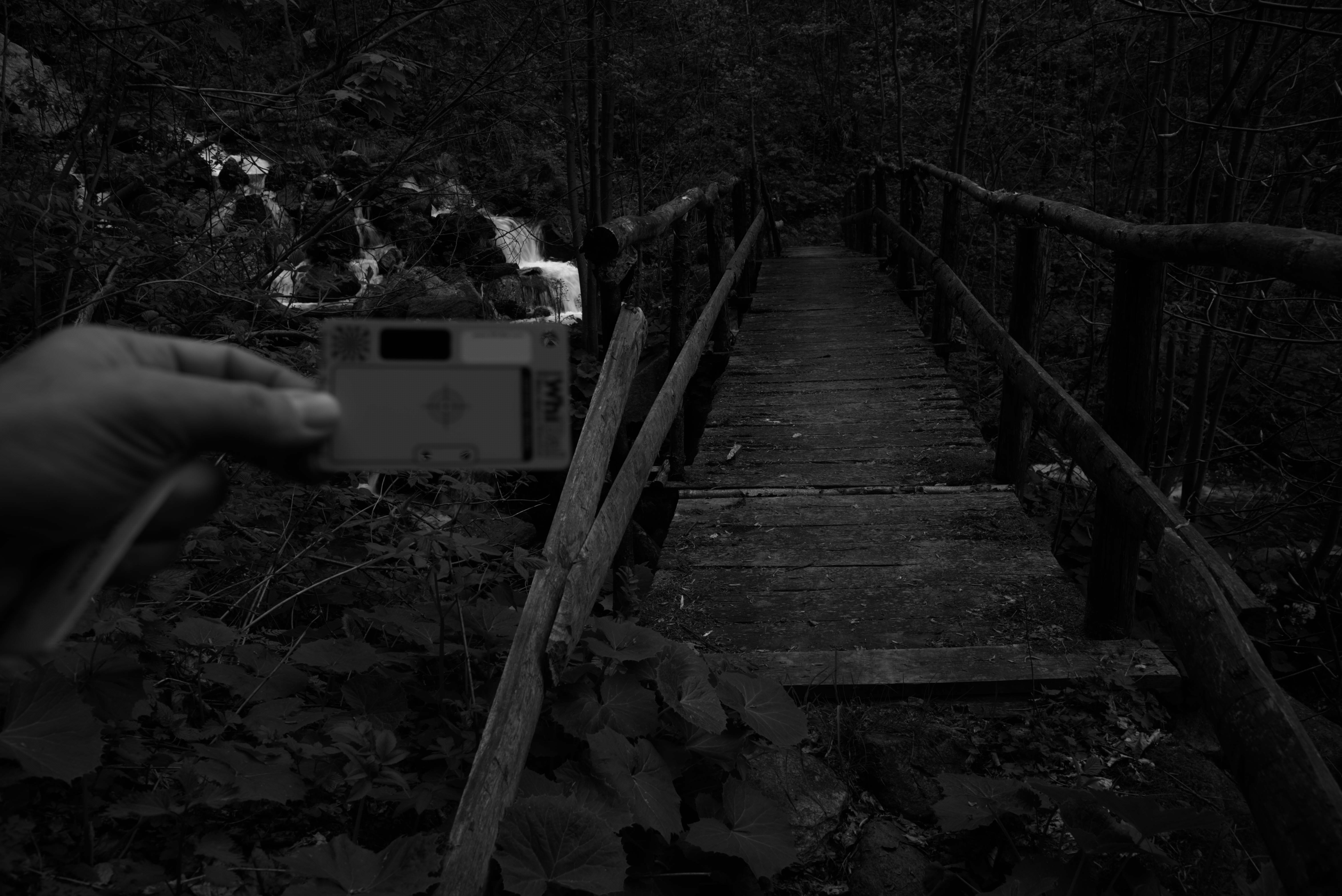
Fig. 3: Step 1: Linear raw image with black levels subtracted. It should look as bright as the following pic. 4. If not, your browser does not handle colors correctly (I am using Chrome and it obviously does not handle them correctly).



If the photo is black, then your browser does not know how to display correctly labeled line data. Interestingly, the WordPress editor displays the image correctly, but after being posted to Chrome, it doesn't look right (note: this was finally fixed by 2019) [2016 article / approx. transl.]. This is how this image should look:





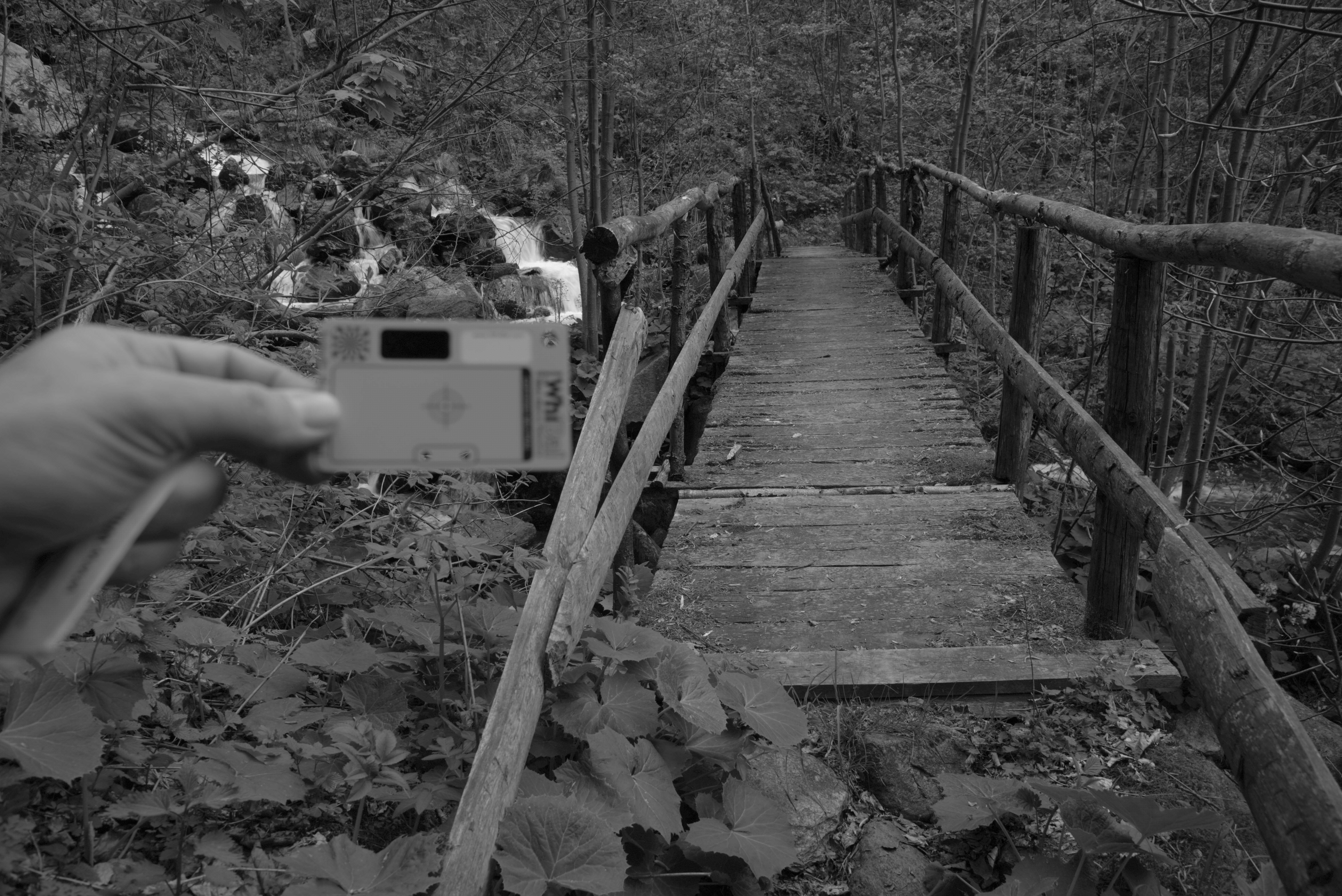
Fig. 4: same photo, but as CFA grayscale



This is how the linear CFA data looks directly in the file. It looks a little dark, since I shifted the exposure to the right so as not to cut off the highlights of the waterfall - we will fix this later, in the linear brightness adjustment step.



The image looks like a full-fledged black and white due to its small size, but in reality it is not: even in equally illuminated areas, pixelation is visible. This is due to the fact that neighboring color filters, having different spectral sensitivity, collect different information about the colors. This is easily seen when enlarging the image. This is what the area of ​​the image just below the WhiBal card looks like at up to 600% magnification:





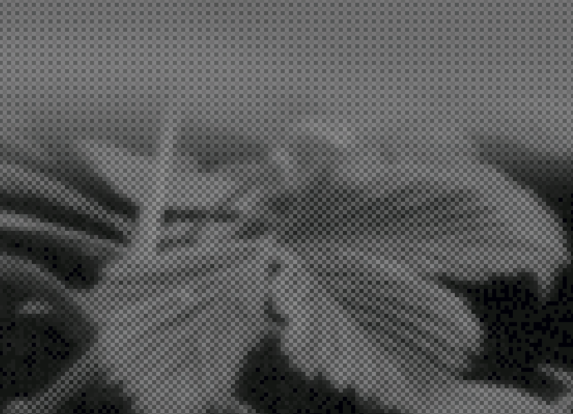
Figure 5: CFA pixelation is visible on a uniformly gray card (top) and on colored leaves.

2. White balance data

Due to the spectral distribution of the energy of the light source (in this case, the sky is partially covered by clouds, the light of which penetrates through the foliage) and the spectral sensitivity of the filters located on the matrix, different colored pixels record proportionally higher or lower values ​​even under the same lighting. This is especially evident in the neutral parts of the image, where it would seem that the same average values ​​should appear over all color planes. In this case, on the neutral gray card, the red and blue pixels recorded values ​​of 48.8% and 75.4% of the green value, respectively, so they appear darker.



So the next step is to apply white balance to the linear CFA data by multiplying every red pixel by 2.0493 (1 / 48.8%) and every blue pixel by 1.3256 (1 / 75.4%). In Adobe terms, we get a black and white image that is neutral to the camera. Then it is guaranteed, with the exception of noise, all pixels will show the same linear values ​​on neutral parts of the image.





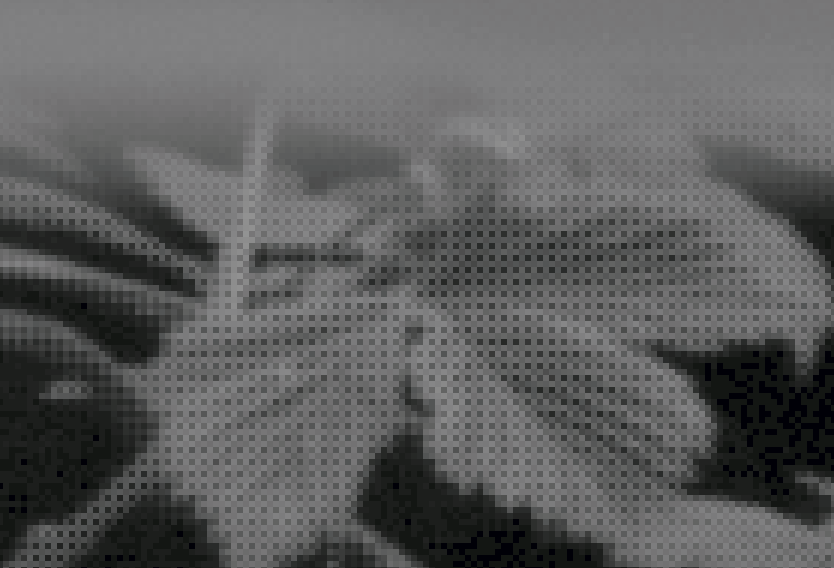
Figure: 6: After white balancing, the pixelation of the gray card disappears, but it is still visible on colored objects.



See how the pixelation at the top of the image disappeared - a neutral gray card was used for calibration. But, of course, pixelation has not disappeared from color objects: information about colors is stored in the difference between the intensities of the three channels.

3. Correction of linear brightness

Most modern digital cameras with interchangeable lenses provide raw data in 12-14 linear bits. The standard bit depth of files (jpeg, TIFF, PNG) is usually set as a multiplier of 8, and 16 bit is the favorite depth of most editors today. We can't just take 14-bit data with subtracted black levels and store it in 16 bits - everything will fall into the bottom 25% of the linear range and be too dark. Ideally, we want to trim the data after white balancing and black subtracting to fit the trimmed data in a 16-bit file, and scale it accordingly (see step 4). A simple way to roughly cast the data is to simply multiply the 14-bit data by 4, scaling it to 16 bits. This is exactly what was done in step 1 after subtracting black (dcraw -d -4 -T does this automatically,and with unprocessed_raw you will need to do it manually).



Speaking of scaling, we might also want to tweak our brightness. This step is subjective and probably not worth doing if you are after an "honest" rendering of an image, such as it came out on the sensor and recorded in a RAW file. However, no one is able to get the perfect exposure, and different cameras often measure average gray at different percentages of the raw data, so it is useful to be able to tweak the brightness. Therefore, many converters refer to the relative sliders as "exposure compensation" or "exposure compensation". Adobe has an associated DNG label that normalizes the exposure meter for different cameras, BaselineExposure. For the D610, it is 0.35 steps.



Our image is a bit dark for my taste, and the WhiBal card, which should be 50% reflective, is only 17% at full scale. Linear luma correction is the multiplication of each pixel in the data by a constant. If we consider that in this image we do not need to preserve the brightest areas of the image with a brightness higher than 100% of scattered white light, then this constant in this example will be 50/17, approximately 1.5 correction steps. In this case, I decided to apply a subjective-conservative correction of +1.1 linear brightness steps, multiplying all the data in the file by 2.14, and the following was obtained:





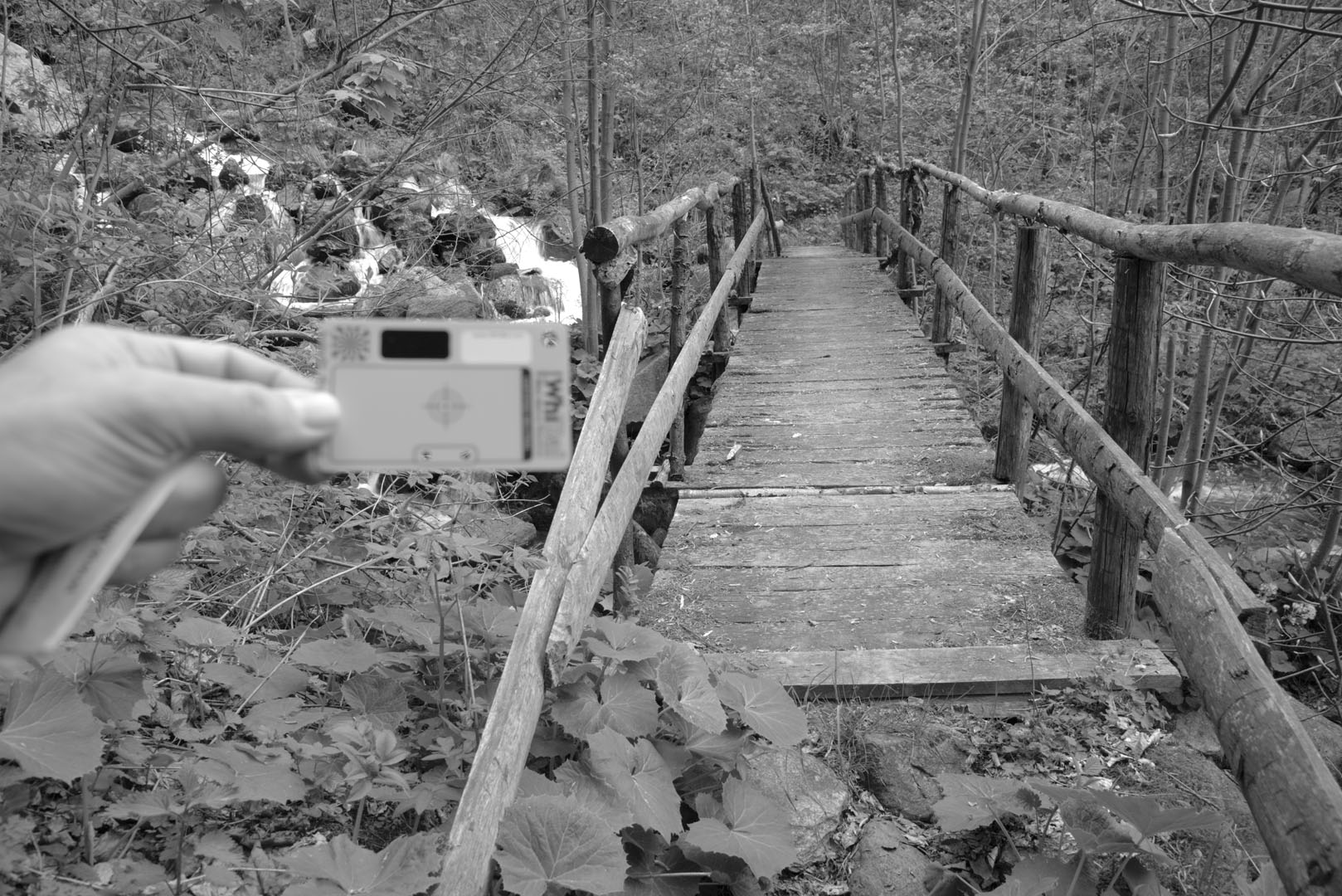
Fig. 7: CFA image after black levels subtraction, white balancing, cropping, linear brightness correction by 1.1 steps



Better. But as you can see, the price to be paid for linear brightness correction is by illuminating parts of the waterfall. This is where the advanced nonlinear highlight and shadow recovery sliders found in most RAW converters come to the rescue.

4. Make sure white balance data is trimmed evenly

If the green channel was initially clipped in the raw data, you may need to crop the other two to full scale after applying white balance multipliers to correct the resulting nonlinearity. The full scale is shown in the histograms below as a normalized value of 1.0. You can see that the green channel of the original raw data was clipped (due to the jumble of values), and the others were not.





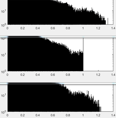
Figure: 8: Top to bottom: R, G, B histograms after applying white balance multipliers to the raw data, before cropping. Be sure to crop all three to the level of the smaller channel so that false colors do not appear in bright areas. The image data is plotted at 0-1, where 1 is the full scale.



Cropping at full scale is necessary because in areas where there is no data from all three channels, the resulting color is likely to be incorrect. In the final image, this can manifest itself as, say, a pinkish tint in areas close to maximum brightness. This is very annoying, for example, in pictures of snow-capped mountains. Therefore, pruning solves this problem uncompromisingly.





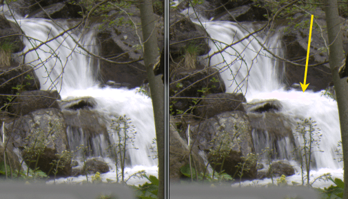
Figure: 9: Left: Correctly cropped image after applying white balance. Right: Image is not cropped. The yellow arrow shows an area close to the maximum brightness, where incomplete information from the color channels gives a pinkish tint.



Instead of cropping, one could make certain assumptions about the missing colors and supplement the relative data. In advanced RAW converters, this is done by algorithms or sliders with names like "highlight reconstruction". There are many ways to do this. For example, if only one channel is missing, as in the case of green from 1.0 to 1.2 in Fig. 8, it is easiest to assume that the highlights are in the neutral white area and the raw image data has the correct white balance. Then, in any quartet where the green color will be cut off, and the other two will not be, then the value of green will be equal to the average value of the other two channels. For this shot, this strategy would be able to reconstruct no more than 1/4 of a step in bright areas (log ₂(1,2)). Then it would be necessary to compress the highlights and / or re-normalize the new full scale to 1.0.

5. Debayering CFA data

Until now, the CFA image was located on the same black and white plane, which made the colored areas appear pixelated, as seen in Fig. 6. It's time for debayering - separating the red, green and blue pixels shown in fig. 2, into separate full-size color planes, by approximating the missing data (in the figure below, they are shown as white squares).





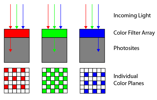
Figure: 10: Debayering - filling in missing data in each color plane using information from all three planes.



Any of a large number of advanced debayering algorithms can be used in this step. Most of them work very well, but some are better than others, depending on the situation. Some RAW converters like open source RawTherapee and dcraw prompt the user to select an algorithm from a list. Most converters do not provide this option, and use the same debayering algorithm. Do you know which debayering algorithm your favorite RAW converter uses?



In this test, I decided to cheat and simply compress each RGGB quartet into a single RGB pixel, leaving the R and B values ​​for each quartet as they were in the raw data and averaging G over two (this is equivalent to dcraw –h mode). It is a 2 × 2 nearest-neighbor debayering algorithm. It gives an image that is half the size (in linear dimensions, or four times in area), which is more convenient to use.





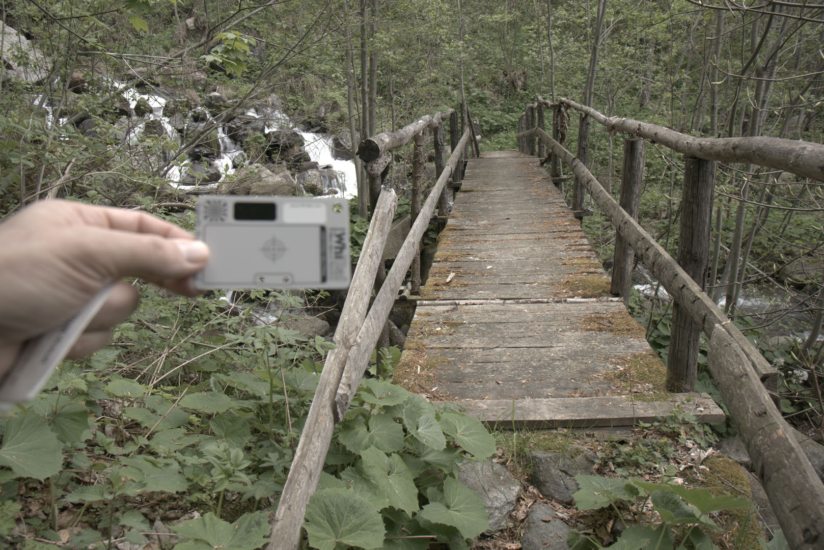
Figure: 11: Raw RGB image after black subtraction, white balancing, cropping, linear brightness correction, and 2x2 nearest neighbor debayering (equivalent to dcraw –h).



In fig. 11, you can see that our raw data is now RGB with three fully filled color planes. The colors, which were recorded by the camera, were shown by the browser and the monitor. They look dull, but not much different from the original. Shades are not stored in standard RGB space, so software and hardware don't always know what to do with them. The next step is to convert these colors to a common colorimetric standard color space.

6. Color conversion and correction

This is one of the least intuitive but most important steps required to get a finished image with pleasing colors. All manufacturers jealously keep the secrets of their color filters in the CFA of their matrices, but with the right equipment it is not too difficult to derive spectral sensitivity functions. You can get a rough idea of ​​the functions of your camera even with a cheap spectrometer .



Armed with all of this, and making a lot of assumptions about typical light sources, scenes, and viewing methods, a compromise linear array can be generated that converts the color from a CFA image (such as shown in Figure 11) to a standard color, which is will be able to recognize common programs such as editors or browsers, as well as devices such as displays and printers.



Fortunately for us, several excellent laboratories are engaged in measuring and calculating these matrices - and then they put the calculations in the public domain. For example, DXOmark.com produces matrices for converting raw photo data after white balancing to sRGB for two sources for any camera in their database. For example, here is their sensor for Nikon D610 andD50 standard light source :





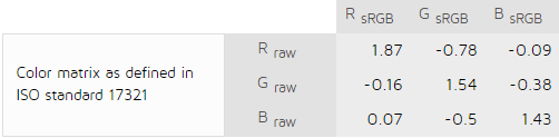
Figure 12: DXO lab color matrix for D50 light source: from white balanced and debayerized data to sRGB.



Which of the compromise matrices will be the best depends on the spectral distribution of the energy of the light source at the moment of taking the frame, so the real matrix is ​​usually interpolated based on a couple of references. In the Adobe world today, these are the standard light sources A and D65, responsible for limiting the range of typical lighting in everyday photography, from tungsten to daylight and indoor photography. The converted data is then adapted to a light source that matches the final color space - for sRGB, for example, D65. The result is a kind of matrix, such as the one shown in Fig. 12. Then all that remains is to multiply it by the RGB values ​​of each debayerized pixel after step 5.



In the specificationAdobe recommends a more flexible process for its DNG Converter. Instead of a direct transition from the CFA camera to the colorimetric color space, Adobe first converts the data to the Profile Connection (XYZ D50) color space, multiplying the data after white balancing and debayering by an interpolated forward matrix, and then comes to the final color space like sRGB. Sometimes Adobe also applies additional nonlinear color correction using special profiles in XYZ (in DNG language, these are HSV corrections through ProPhoto RGB, HueSatMap and LookTable).



The direct matrices of the camera that took the picture are recorded in each DNG file, praise Adobe. I downloaded the matrices for D610 from there, and matrices XYZD50 -> sRGBD65 from Bruce Lindblum's site , and gotFinal image:





Fig. 13: "Fairly" converted image. Raw data, black levels subtracted, white balancing performed, cropping, brightness corrected, 2x2 debayering, color corrected and converted to sRGB.



Now the colors are what programs and devices expect to find in the sRGB color space. In case you're wondering, this image is almost identical to that of Nikon's Flat profile Capture NX-D converter. However, it does not look very sharp due to the poor contrast of our monitors (see Tone Mapping).

7. Application of gamma

The last step depends on the selected color space. The gamma for sRGB space is about 2.2 . I only mention this specifically to show that the rendering process becomes non-linear at this point. From this moment on, the image is reduced to the colorimetric gamut of the color space, and it can be either loaded into your favorite editor or displayed on the screen. In theory, all the previous steps were linear, that is, easily reversible.

+ Tone display

In 2016, tone correction is almost always required to determine how to squeeze the high dynamic range of the camera into the small range of the imaging device. For example, depending on your resistance to noise, the dynamic range of my D610 has 12 steps, while my quite good monitor has a contrast ratio of 500: 1, or about 9 steps. This means that the bottom three steps from the camera will not be visible on the monitor due to its backlight.



The RGB curve will subjectively redistribute the tones across the range, so that some shadows are more visible at the expense of some of the brightest areas (hence this curve is called the "tone curve"). At the time of this writing, such a curve is usually applied by Adobe in ACR / LR at render time, before showing the image for the first time:





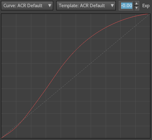
Figure: 14: Tone curve applied by ACR / LR near the end of the rendering process in Process Version 3 (2012-2016). The horizontal axis is non-linear.



In this case, I didn't use it. I just applied a curve of increasing the contrast and added some sharpness in Photoshop CS5 to fig. 13 to get the final image:





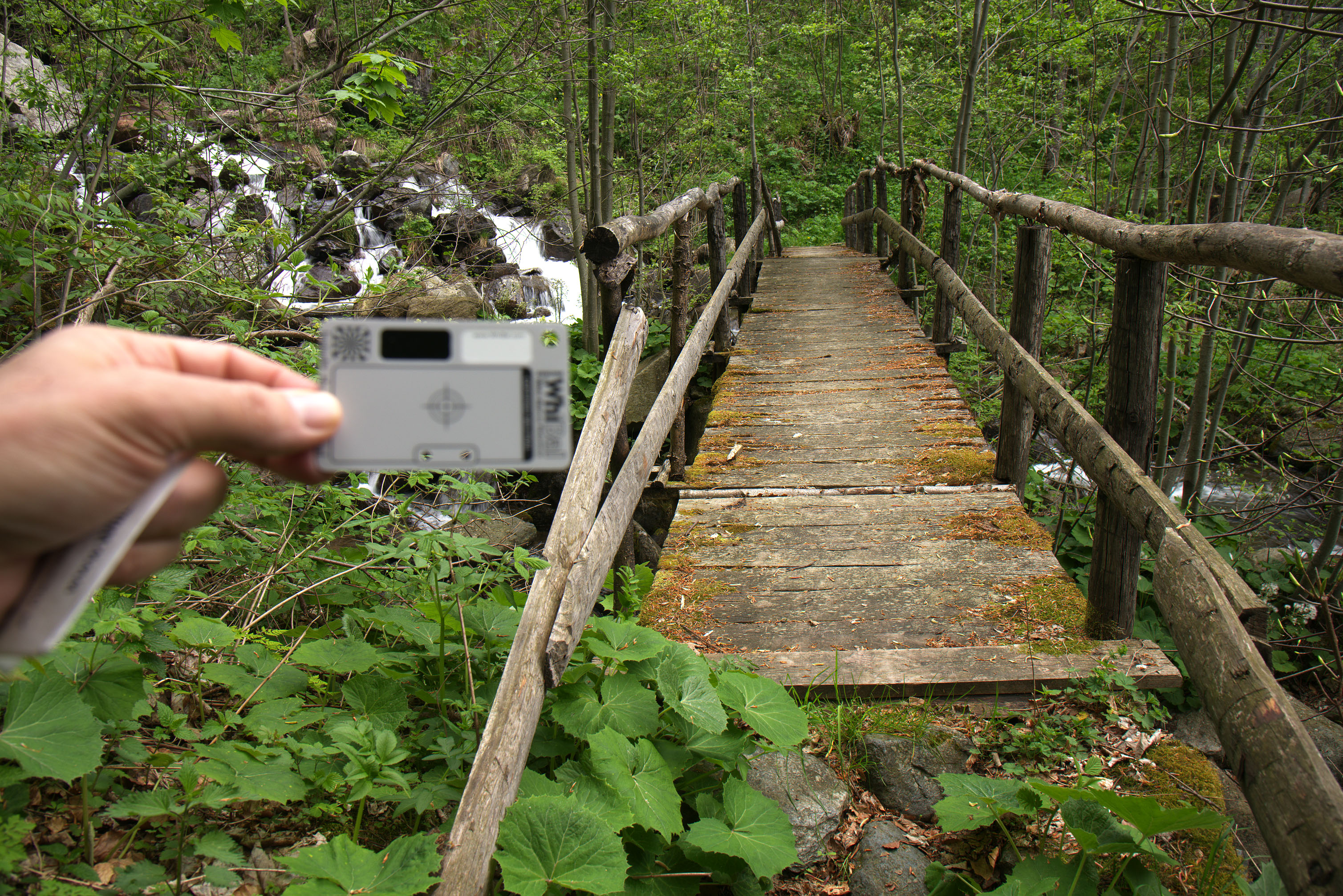
Fig. 15: Final sRGB image. Initial raw data, black levels subtracted, white balancing, cropping, brightness tweaked, debayering, color tweaked, tone curve applied



Of course, applying a contrast curve at a later stage changes the chromaticity and saturation of the colors, but this is exactly what happens when you apply these adjustments to the RGB gamma space after rendering the image. Historically, this is how everything happened in cameras, and this is how everything happens in popular RAW converters - this is the procedure, and we got used to it over the years. An alternative to achieve "accuracy" of color reproduction will be to use the color profile from the Torgera website, and no longer touch the tone.

Let's summarize

So, for basic RAW conversion with linear adjustment of brightness and color, you need:

1. Load linear data from RAW file and subtract black levels.
2. Balance white.
3. Correct linear brightness.
4. Crop image data.
5. Debayerize.
6. Apply color transformations and corrections.
7. Apply gamma.

And that's all - the veil of secrecy from the conversion of raw data has been torn away.



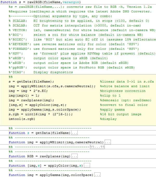
Scripts for Matlab for obtaining the images given in this article can be downloaded from the link . The 7 basic steps are marked in yellow:



s = raw2RGB(‘DSC_4022’ , ‘ROI’ , 1.1)



After using the script, save the file in TIFF format, load it into the color editor and apply the chosen color space to see the correct colors.