Filipp Titarenko, Product Manager for Femap, Nanosoft JSC
Introduction, or Why and what this article is about
Not all engineers know how to solve nonlinear analysis problems. And for many, even among those who specialize in calculations in finite element analysis programs, the phrase "nonlinear analysis" is misleading or even frightening. Those who have tried to solve such problems in passing recall windows with a large number of settings and some graphs that move somewhere and at the same time something "does not converge" (Fig. 1). However, not only scientific problems, but also modern engineering norms and standards often require taking into account nonlinearity in calculation models. Moreover, these requirements exist not only in the space, aviation, engineering industries. So, for example, the set of rules of the joint venture 385.1325800.2018 "Protection of buildings and structures from progressive collapse" when carrying out calculations requires taking into account the geometric and physical (plasticity, creep, etc.) nonlinearity.

Picture 1
The statistics for today are such that about 90% of calculations fall on linear analysis. From an economic standpoint, linear analysis is fast, simple, and cheap. But if you need to calculate the response to the impact of shocks, take into account inertial effects, trace the change in temperature or other parameters over time, take into account the presence of contact surfaces, geometric nonlinearities or complex mechanisms of material behavior, you cannot do without nonlinear analysis and the ability to correctly configure the solver. The main types of nonlinearity are physical geometric and due to the presence of contact surfaces.
On the Runet (and in the global network), there are two conditional types of educational materials on the topic of nonlinear finite element analysis: 1) not too long instructions on where and in what sequence to click in your CAD system to calculate your "beam, heating, bracket, current ... ", or 2) thick college textbooks / scientific papers or multi-page user manuals that can and should be studied for a long time ... but in the coming days and weeks it is unlikely that it will be possible to calculate something on your own.
This article is an attempt by the author, using a specific example in a specific CAD system, to illustrate the algorithm for carrying out nonlinear static analysis from scratch to analysis of the solution, while offering some explanations of the theoretical foundations associated with the solver settings.
We will solve the problem in the Femap pre-postprocessor with the NX Nastran solver, which has proven its reliability, accuracy and speed since the mid-70s of the last century. I use Femap 2020.2, but in general the algorithm for solving this kind of problems is identical not only in previous versions of Femap, but also in other FE computational complexes.
What will we train on? Nonlinear static analysis
No, unlike the hero of the old comedy movie (Fig. 2), we will not train on cats.

Figure 2
We have to calculate the L-shaped bracket beyond the yield strength of steel. A real prototype of the bracket can be a climbing bolt, a bracket on the ISS, or an element of a hinged ventilated facade. I chose it because, on the one hand, I did not want to take the finished model, and on the other hand, it would be nice not to spend a lot of the reader's time on the process of creating geometry. From the point of view of the model, everything will be as simple as possible, I will pay more attention to the theory and solver settings. With this approach, the reader will have the opportunity to independently repeat the entire process - from creating a model to its numerical analysis. And even conduct a natural experiment.
In the process of preparing the article, I discovered at my home a similar, but perforated bracket (Fig. 3), which I had previously removed with pliers beyond the yield point - albeit with different boundary conditions for fixing. And for other purposes - not scientific and experimental, but for household purposes ...
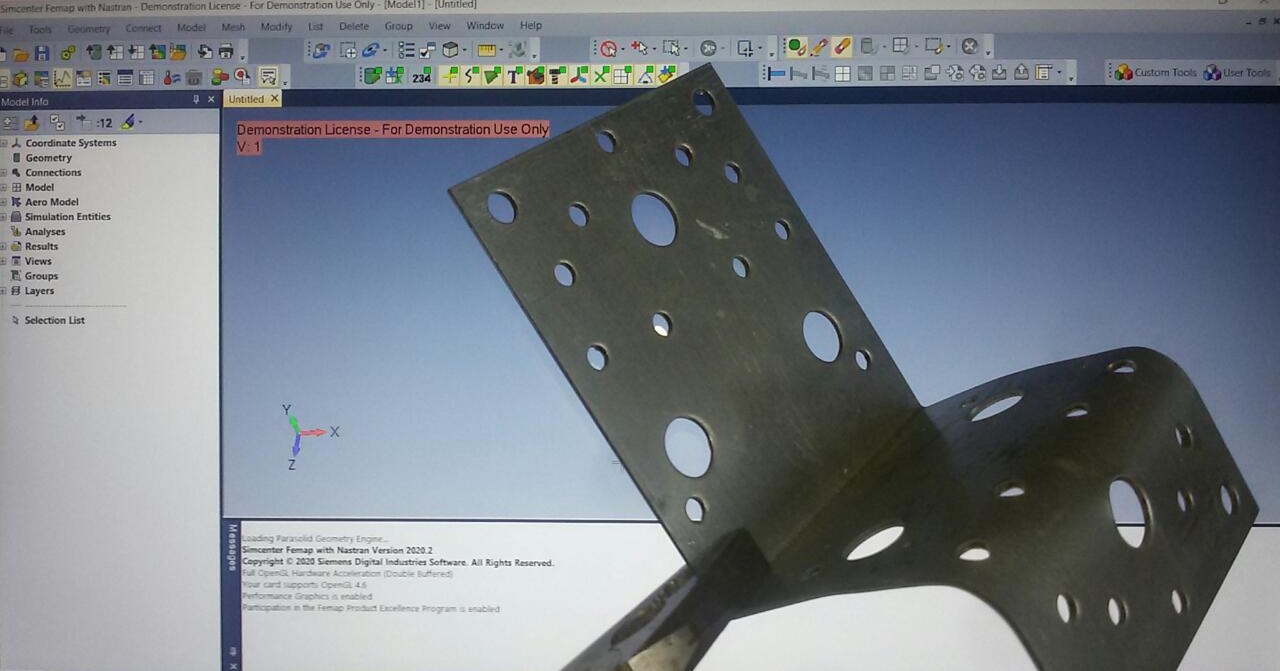
Figure 3
But if you wish, you can always verify your numerical experiment: such brackets are available in all hardware stores.
A bit of theory: the differences between linear and nonlinear analysis
For the practice of solving engineering problems from the point of view of internal computational algorithms, it is important to realize that in nonlinear analysis loads are applied gradually and in fact the solver consistently solves many problems. In linear static analysis, only one step is always taken: from the initial state to the final state. When solving a nonlinear problem, all specified loads will not be applied to the body immediately.
The initial data for each subsequent step in nonlinear analysis is the state of the model at the previous step. Moreover, at each step, the internal and external forces (energy parameters) must be balanced, taking into account some error (Fig. 4). The amount of permissible error is determined by the Convergence Tolerances criterion. Typically, this criterion is set as a percentage of the applied load, where the load refers to all external forces applied to the model or, in the case of displacement loading, reaction forces. The abundance of settings is explained by the complexity of the computational algorithms accompanying nonlinear analysis. The typical value of the force convergence criterion ranges from 0.1 to 1% of the applied load. In searching for convergence at a solution step, the program can perform many iterations.For these reasons, solving nonlinear problems takes much more computer time than solving linear static problems. It is important to realize that the multistep approach may, for various reasons (types of nonlinearities), require problems, the result of solving which does not depend on time.
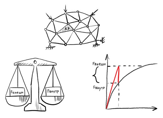
Figure 4
The simplest example on which this statement can be understood is the loading of an elastic-plastic structure with a load at which the stress exceeds the yield point. The solver "does not know" in advance at what load the stress in individual nodes of the model will exceed this limit and, therefore, the parameters of the equations describing the stress-strain state of the body will fundamentally change. In this case, at each step of the force increment, it is necessary to take into account the change in the plastic deformation zone. Therefore, the solution goes through many steps of increasing the load, and the steps, in turn, if necessary, are performed for a certain number of iterations. Stiffness matrix calculations can be repeated at each solution step. The recalculation frequency of the stiffness matrix is set by the user. Plasticity is physical nonlinearity.
Due to the “multi-step” and “iterative” solution process, I recommend that you master the Nonlinear History tab, which you can go to by running the solver. In it, you can track the number of iterations performed and the level of the load achieved (Load Factor) in real time according to the schedule. From this graph, you can analyze the rate of convergence of the solution. If something goes wrong, the solver will interrupt the solution process and display a message that the solution does not converge.
Linear analysis can only be used to analyze models with linear materials, provided that there are no other types of nonlinearities. Linear materials can be isotropic, orthotropic, or anisotropic. If the material in the model has non-linear stress-strain characteristics under a given load, non-linear analysis should be used. Various types of material models can be used in nonlinear analysis.
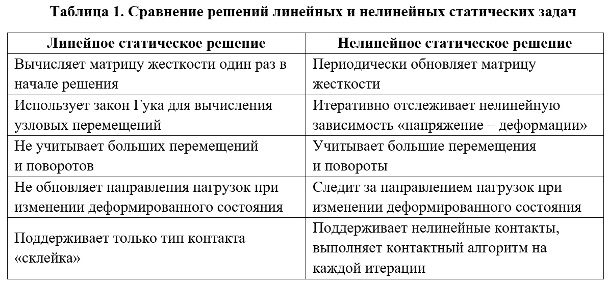
In a nonlinear static analysis, dynamic phenomena like inertial forces and damping forces are not taken into account. The processing of a nonlinear static solution differs from the processing of a linear static solution in several main points, presented in table. 1.
The general theory is enough for this, but I will write below about how to set up the algorithms for solving the global nonlinear system of algebraic equations generated by the finite element method, when we get to the appropriate place when analyzing our practical example with a bracket. In Femap, most of these settings are found in the Nastran Nonlinear Analysis dialog, which can be accessed from the Analysis Set dialog by setting 10..Nonlinear Static in the Analysis Type field and clicking Next several times. But everything has its time.
Getting Started: Bracket Modeling and Linear Analysis in Femap with NX Nastran
In the command menu open File → Preferences → Geometry / Model tab. In the Solid Geometry Scale Factor settings, set Meters, which corresponds to the SI system of measurements of physical quantities.
Our L-shaped bracket will consist of two square plates with sides of 0.1 meter, located in perpendicular planes. In the command menu, go to Geometry → Surface → Corners and successively create two square plates.
1) The coordinates of the vertices for the first plate: 1) X = 0; Y = 0; Z = 0; 2) X = 0.1; Y = 0; Z = 0; 3) X = 0.1; Y = 0; Z = 0.1; 4) X = 0; Y = 0; Z = 0.1.
2) For the second: 1) X = 0; Y = 0; Z = 0; 2) X = 0; Y = 0.1; Z = 0; 3) X = 0; Y = 0.1; Z = 0.1; 4) X = 0; Y = 0; Z = 0.1.
By sequentially driving these points into the Locate → Enter № Corner of Surface dialog box, we will get the desired geometry. By pressing Ctrl + A, we can display our geometry in the center of the viewport at a convenient scale.
Next, we will create the material of our plates (Steel 3) and define its properties. To do this, in the Model Info panel located on the left side of the screen, open the Model tab, then right-click on the Materials line and click New. The Define Material - ISOTROPIC dialog box opens. In the Title field, enter the name St3. In the General field, set Young's Modulus, E = 2e11, Poisson's Ratio, nu = 0.3, Mass Density = 7850. We won't go to the Nonlinear tab for now. Click OK and then Cancel.
Let's create an end element type and specify its properties. To do this, in the Model tab, right-click on the Properties line and click New. The Define Property - Plate Element Type dialog box opens. In the Title field, enter the name Pl0005. In the Material tab, select 1..St3. Then click the Elem / Property Type button and make sure the checkbox is in the right place: Plane Elements - Plate. That is, a flat finite element is selected - a plate. Let's set the thickness of the plate, for this, in the Thicknesses field, set TavgorT1 = 0.005. Click OK and then Cancel.
Let's save our model, for which we press File → Save As, select the path to save the file and the file name. I'll call it KronNonlin.
Let's set the mesh properties of the finite element model. To do this, in the command menu, click Mesh → Mesh Control → Size On Surface. In the Entity Selection → Select Surface (s) to Set Mesh Size dialog box, click Select All to select all surfaces. Clicking OK, we get into the Automatic Mesh Sizing dialog box. In the Element Size field, set the value 0.005 and click OK. Now the characteristic dimension of our finite elements will be 5 mm. Points appeared on the lines of the model, giving us information about the size of the elements after creating the finite elements.
Now let's create a finite element model. In the command menu, click Mesh → Geometry → Surface. In the Entity Selection → Select Surfaces to Mesh dialog box, click Select All and OK. In the Property field, set the FE type we created 1..Pl0005, and in the Mesher field, set the Quad checkbox. Click OK. The finite element model has been created. Now we will fix the bracket and load it with external forces.
We will fasten the bracket for four nodes (such fastening most closely corresponds to fastening with rivets or spot welding) along six degrees of freedom, and along the line of the joint of two plates - along three degrees of freedom (leaving the possibility of rotation around the line).
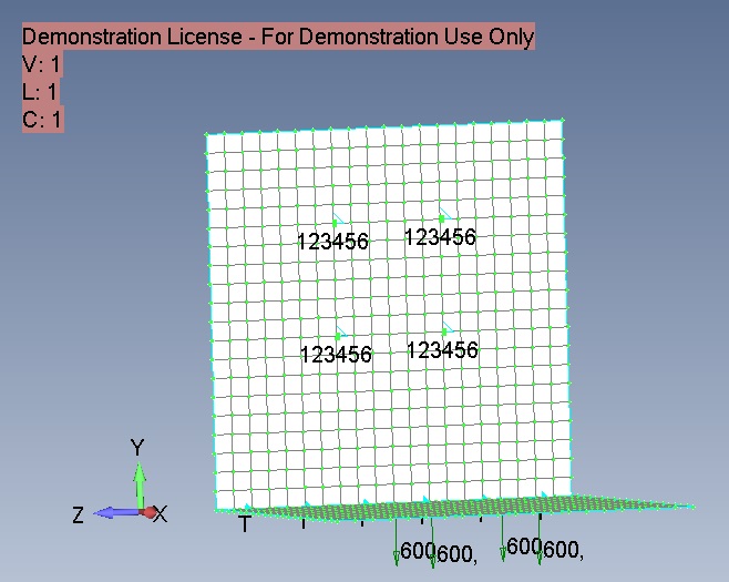
Figure 5
We set the boundary conditions for fixing. To do this, right-click on Constraints, click New and enter the name Constr. Next, right-click on Constraints Definitions and select Nodes. Selecting four nodes as shown in fig. 5, we fix them in six degrees of freedom; click OK. In the Title field of the Create Nodal Constraints / DOF dialog box, write 4nodes and click on the Fixed button to constrain movement-rotation. Click OK. Right click on Constraint Definitions again and select Curves. In the Title field of the Create Constraints on Geometry dialog box, specify Line and click the Pinned - No Translation button to constrain the movement, leaving the possibility of rotation.
Let's set the loading conditions by right-clicking on Loads - New. The new Set will be called Vert. Right click on Load Definitions - Nodal and select four nodes to which the load data will be applied. In the Create Loadson Nodal dialog box, let's name our load Force600. Nodal forces are directed along the Y-axis in the negative direction. The value of the nodal load FY is minus 600 Newton. Thus, a load of 600 Newtons will be applied to each of the four nodes (i.e. 240 kg for all four nodes).
Next, go to the analysis settings. In the command menu, select Model → Analyzes. Press the New button to select the analysis type and solver. In the Title field, enter Linear. We select the Analysis Program - 36..Simcenter Nastran and Analysis Type 1..Static. Then, by clicking on the Analyze button, we start the calculation. The solution takes me less than one second (!). Femap shows us a window for observing the analysis results: Simcenter Nastran Analysis Monitor. Analysis complete line 0 means that the analysis was completed successfully.
In Model Info, right click on Results → All Results → Deform. Now we see the deformed state of our bracket in an exaggerated form. In my opinion, the deformed state is visually exaggerated, so press F6 and the View options dialog will open. Let's go to the PostProcessing tab, Deformed Style in the Scale field, set 4%. The visualization of the deformed state of the model is now less exaggerated. The maximum displacements can be viewed in the lower left corner of the model - they are 0.0026 m.
Press the F5 key and display the stress distribution across the model. In the Contour Style field, check the box for Contour, then click the Deformed and Contour Data button. In the Contour tab, select 7033 Plate Top Von Mises Stress so that Femap will display the stresses at the nodes. Our model has become multi-colored, the colors reflect the level of tension (Fig. 6). On the right side of the screen, we see a scale showing which color corresponds to which voltage level. To hide the geometric original model, click on the View Surfaces Toggle icon. The maximum stresses reach 332.4 MPa, which is significantly higher than the yield point of 210 MPa for St3 steel.
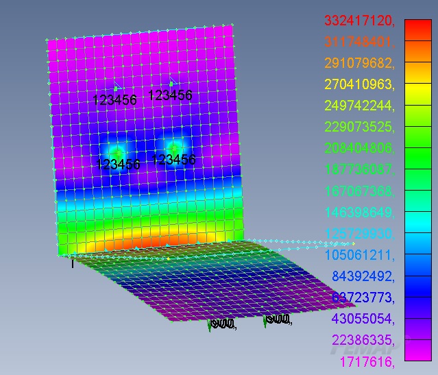
Figure 6
So, the stresses at the points of the bracket are much higher than the yield point. Linear analysis does not take into account the fluidity-plasticity of materials and the effect of stress redistribution associated with this phenomenon, therefore this stress distribution does not correspond to reality. Let's move on to nonlinear analysis.
Practice: Nonlinear Static Analysis in Femap with NX Nastran
To move from a linear to a nonlinear model, we need to perform just a couple of actions (we do not change the partition, the conditions of fixation and loading).
Change the properties of the material by adding plastic deformations; to do this, in the Materials tab, right-click on our material 1 ... St3 and press Edit. Let's go to the Nonlinear tab and select Plastic in the Nonlinearity Type field. In the Yield Criterion field, select 0..von Mises, in the Initial Yield Stress field, enter the value 210,000,000 (that is, 210 MPa). Click OK.
NX Nastran supports the following ductility criteria:
- Mises (von Mises) - used for plastic material in most cases;
- Cod (Tresca) - for fragile and some ductile materials;
- Drucker-Prager - for materials such as soil and concrete with internal friction;
- - (Mohr-Coulomb) – .
- .
In the command menu, select Model → Analyzes. Press the New button to select the analysis type and solver. In the Title field, enter Nonlinear1. We select the Analysis Program - 36..Simcenter Nastran and Analysis Type 10..Nonlinear Static. Click the Next button. In the Nastran Executive and Solution Options window, check the Number of Processors box and enter the number of processors on our computer. Then we press the Next button six times in a row, without changing the default settings in the dialog boxes, until we get to the Nastran Nonlinear Analysis dialog box. This is the key window for nonlinear analysis settings, so let's dwell on this place in more detail and consider its settings fields (Fig. 7).
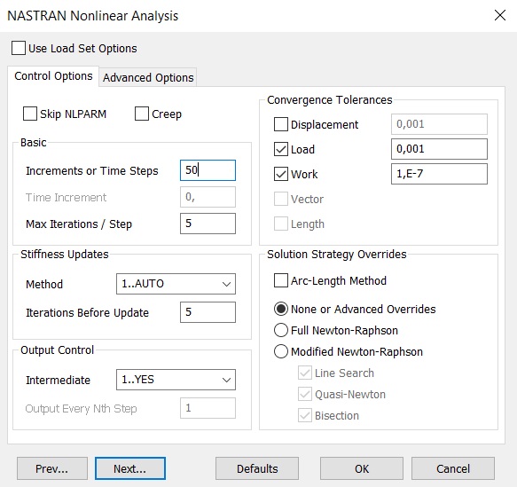
Figure 7
If it is necessary to take into account the effect of creep, check the Creep box.
In the Basic field, set the number of steps for increasing the load (Increments or Time Steps) and the maximum number of iterations at each step (Max Iterations / Steps). In the case of nonlinear static analysis, Increments or Time Steps reflect the load level. In the Nonlinear History graph, which illustrates the number of iterations performed in real time, the load level is plotted on the vertical axis and is called the Load Factor. Its value lies in the range from 0 to 1. For a given number of steps, the load changes from 0 to full; in this case, if the convergence conditions require it, several iterations are performed within one step. These two parameters are very important, in each task you should try to choose a “golden mean” between too many “steps” and “iterations” and too few. If there are too few of them,then the solution will not converge or will have a negative impact on accuracy. If their number turns out to be excessive, the solution will consume a lot of machine power, time, and convergence may be negatively affected. To investigate the influence of these parameters, we solve our problem with a bracket several times with different combinations of the number of "steps" and "iterations", while observing the graph of non-linear chronology.while observing the non-linear chronology graph.while observing the non-linear chronology graph.
For a nonlinear static problem in the Stiffness Updates field, you can select one of three methods (AUTO, ITER, SEMI) for updating the stiffness matrix of the body, as well as the number of iterations (Iteration Before Update) through which the matrix will be updated. If the method is chosen incorrectly, then 0..Default (by default) will be used automatically. In the AUTO method, the stiffness matrix is updated based on the estimates of the convergence of different numerical methods (quasi-Newtonian, with linear iteration, half division) and with the choice of the one that will give the minimum number of updates to the stiffness matrix. The SEMI method is similar to the AUTO method, but the stiffness matrix is necessarily updated at the first iteration after changing the load, which is effective for highly nonlinear processes.The ITER method (in nonlinear time analysis it is similar to the TSTEP method) updates the stiffness matrix after the number of iterations specified in the Iteration Before Update field. The ITER method is effective for highly nonlinear processes in which the geometry of the body changes dramatically during deformation (for example, when stability is lost).
In the Output Control field, the settings for outputting the results at intermediate loading steps (time steps, if we are talking about time analysis) are specified. When performing static nonlinear analysis in the Intermediate tab, you can select one of the following options: 0..Default (default), YES (display), NO (do not display), All (display at all steps). With nonlinear analysis in time, you can set the number of steps after which the result should be displayed.
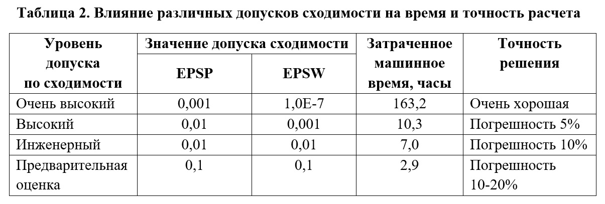
The Convergence Tolerance field specifies the tolerances for meeting the convergence conditions for loads (Load), displacements (Displacement), and internal work (Work). Let us consider the influence of the Convergence Tolerances on the accuracy and time of solving the problem using the example of the model studied by the developers of Femap with NX Nastran from Siemens.
A very large nonlinear model (950,000 DOFs) was carefully examined to determine the effect of different convergence criterion tolerances on runtime and calculation accuracy. There was no heat transfer, gaps or contacts in this model. The results of the study showed that the acceptable accuracy of the solution (in comparison with the solution obtained with a very high level of convergence tolerance) can be achieved for both the “high” and “engineering” convergence tolerance levels. An estimate convergence tolerance level produces a result with the same general trends as higher tolerance levels, but the answers are not accurate enough for a working draft. With a decrease in the tolerance level for convergence, the calculation is much faster. Table 2, the presented trends can be quantified.
In the Solution Strategy Overrides field, the settings for the process of solving the global nonlinear system of algebraic equations generated by the finite element method are set. To consciously change these settings, you need to have knowledge and experience - if they are not enough, it is better to leave the default settings. Here are some explanations.
Arc-Length Method sets the value of the time step (additional load), taking into account the information about the displacement of the nodes of the body - it should be used if the task is associated with a sharp deformation (loss of stability).
The Full Newton-Raphson method converges very quickly, but it takes additional time to create an additional matrix for the full matrix of the system of algebraic equations at each iteration.
The Modified Newton-Raphson method does not need this action, but converges much more slowly, so additional procedures can be used to speed it up: Line Search (linear search), Quasi-Newton (quasi-Newtonian acceleration) and / or Bisection ( half division).
Thus, we have analyzed the basic settings for nonlinear static analysis (the settings for nonlinear analysis in time are very similar to them). To calculate our bracket in the Nastran Nonlinear Analysis window, set the following parameters: in the Increments or Time Steps field - 50, Max Iterations / Step - 5, Stiffness Updates Method - 1..AUTO, Iterations Before Update - 5, Intermediate - 1..YES ... Leave the rest of the settings unchanged. Click OK and go to the Analysis Set Manager window. To start the calculation, press the Analyze button. Femap will automatically open the Simcenter Nastran Analysis Monitor window. Let's go to the Nonlinear History tab by moving the checkbox from log to Nonlinear History (Fig. 8).
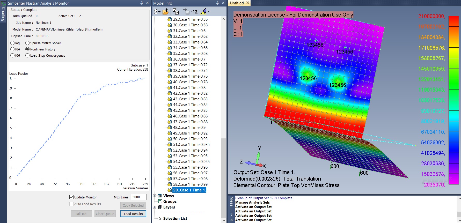
Figure 8
It displays a graph showing in real time the number of iterations performed and (in the case of our nonlinear static analysis) Load Factor, that is, a load factor from 0 to 1. In the upper right corner, we see information about the current iteration number. Please note that this is not the step number of the load increment, but the number of the current iteration. Each step of the load increment can contain several iterations - this is necessary for the execution of algorithms that implement the convergence of the solution. If the increment does not converge, it means that the change in load is too large to proceed to the next step; the load is reduced - additional iterations are performed within one step.
In the Model Info window, open the Results → All Results tab. Double-clicking on the solution line opens the results at various load levels from 0 to 100%. Let's analyze together the graph of nonlinear chronology and the stress-strain state of the bracket at different load levels.
At a load level from 0 to 0.62 (Load Factor), the stress is less than the yield point of 210 MPa, after which plastic deformation of the bracket steel begins. Unit 1 corresponds to a total applied load of 240 kg for four nodes. Maximum stresses are highlighted in red - they are concentrated near the line of intersection of surfaces. At a load level of 0.62 to 1, the plastic deformation zone increases - the maximum stresses (in contrast to linear analysis) do not increase. With a load factor of 0.82, the growth rate of the curve decreases, which means that more iterations are required for each step to satisfy the convergence conditions. We were able to reach full load 1 - the maximum displacement was 0.00283 m. In some cases (for example,if we significantly increased the load), the geometry of the deformed body is distorted so much that convergence cannot be achieved with this strategy (solver settings). As you can see, the results of nonlinear analysis are qualitatively and quantitatively different from the results of linear analysis.
Let's carry out three more calculations, setting different settings for the number of steps of increments and iterations (Fig. 9). In the first case, Increments or Time Steps - 50, Max Iterations / Step - 5 were set.
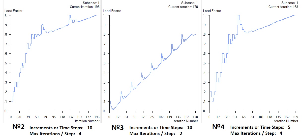
Figure 9
The convergence conditions were met in the 1st, 2nd and 4th calculation cases. In the 3rd design case, a fatal error with the explanation that the solution does not converge appeared at a load level of 0.8. Note that in the 2nd and 4th calculations, the solution was performed successfully (full load 1) with a significantly smaller number of steps and iterations. Our model is simple enough and all calculations were done in less than 5 seconds. On large models, a lot of machine time can be saved by choosing the right number of load increments and iterations.
Conclusion
Many questions remain outside the scope of this article: multistage loading (application of Case and Subcase), application of nonlinear contacts, nonlinear analysis in time, actions in cases when the solution "falls apart". But I hope that the main goal of the article has been achieved - those readers who do not have extensive experience in solving nonlinear problems now have a minimum set of theoretical knowledge and practical images to get started with nonlinear finite element analysis.
Literature
- Basic Nonlinear Analysis User's Guide. Siemens.
- Rudakov K.N. Femap 10.2.0. Geometric and finite element modeling of structures. K .: KPI, 2011 .-- 317 p., Ill.
Philip Titarenko,
Product Manager for Femap
, Nanosoft JSC
E-mail: titarenko@nanocad.ru
Dear readers, I invite you to three interesting and useful events that will take place in the near future:
- On August 20th, I'm hosting a free webinar " Nonlinear Analysis in Femap with NX Nastran ".
- On September 17th I am waiting for you at the webinar "Contact tasks in Femap with NX Nastran". A link to it will appear in the coming days in the events section .
At the webinars, I will be happy to answer your questions. - The Femap Symposium 2020 will be held on September 9 and 10, during which specialists from Russian industrial companies and Femap developers from Siemens will share their engineering experience and skills in the field of finite element modeling. To learn more about the symposium, follow the link .
A free trial version of Femap with NX Nastran can be downloaded here .