Relations. Part I

The formal theory of modeling uses algebraic relations, including them in the signatures of models of algebraic structures, which describe real physical, technical and informational objects, the processes of their functioning. Among the latter I include, for example, databases (relational databases (RDBs)). I consider the area of ​​decision-making to be no less important, which consists of two main statistical and algebraic, based entirely on the theory of relations. The educational level of specialists in this theory is close to zero.



Open the textbook on specialization and there you will see, at best, about equivalences, which are interpreted by the authors in a very peculiar way. I ask one already defended DTN: Do you consider the relation of equivalence by indicating neither the carrier of the relationship, nor a specific relationship, how does it look in your record? Answer: what it looks like - usually. It turns out that he has a very vague idea of ​​all this.



I find it difficult to name publications on the design of a ReDB, except for foreign articles. In the 90s, he was an opponent, wrote a review of a thesis, which considered hierarchical, networked, and relational databases. But once a year, a year and a half ago, work again came to the review, the author writes already only about the DB, about the normalization of DB relations, but did not show any theoretical novelty. Many universities teach a course on databases, but not on how to create them, create a DBMS, but, as a rule, on how to operate a ready-made (foreign) database.



Rev. the staff is not ready to teach IT specialists to create domestic DBMS, OS, programming languages, not to mention LSI, VLSI, custom LSI. Here, apparently, the train left for a long time and for a long time. So in vain some cheeks are puffed up with pride (read snobbery), this can be seen from the comments on other people's publications, show yourself that you can, and do not indulge in useless translations and re-songs of someone else for the sake of pride - "rating" and "karma" Affects not only the lack of creativity, but simple education and upbringing.



The second domain that is inextricably linked to relationships is decision making. Each of us is constantly busy with this. We will not lift a finger without a decision of the conscious or unconscious. Few understand, and even less write about solutions. The decision of any decision maker (decision-maker) is based on the preference for alternatives. And the preference model is precisely this type of relationship, which is called the "space of preference relationships." But who studies them. When I came to a “specialist” in relations with a question about the number of relationships of each type, he, not knowing the answer, “killed” with a counter question, why do you need it?

Relationship concept

I think that the term attitude is familiar to every reader, but asking for a definition will confuse most. There are many reasons for this. They are most often in teachers who, if they used relationships in the teaching process, did not focus on this term, apparently did not cite memorable examples.



In my memory there are several memorable examples for a lifetime. About mappings and relationships. I'll talk about mappings first. There are two buckets of paint. In one white in the other - black. And there is a box of cubes (a lot). The faces have embossed numbers. How many ways can you color the faces of the cubes in two colors? The answer is unexpected - as many as 6-bit binary numbers, or 2 ⁶= 64. Let me explain in more detail f: 2 → 6 2 objects are displayed in 6. Each line of the table is a discrete display of fi.



Let's build a table with 6 columns and the colors will match the number white - zero, black - one, and the faces of the cube are columns. We start with the fact that all 6 faces are white - this is a 6-dimensional zero vector. The second line is one face black, that is, the least significant bit is filled with 1. and so on until the 6-bit binary numbers are exhausted. We put the cubes in a common long row. Each of them seems to have a number from 0 to 63.



Now the display is reversed. A pack of sheets of paper (many) and 6 paints (felt-tip pens).

Mark both sides of the paper sheets with felt-tip pens of different colors. How many sheets are required. Answer f: 6 → 2 or 6 ² = 36. These are arbitrary mappings.



Let's move on to relationships. Let's start with an abstract set - the carrier of the relation

A = {a1, a2, a3, ..., an}.

You can read about it here . For better understanding, we will reduce the set to 3 elements, i.e. = {a1, a2, a3}. Now we perform Cartesian multiplication × = ² ,

× = {(a1, a1), (a1, a2), (a1, a3), (a2, a1), (a2, a2), (a2, a3 ), (a3, a1), (a3, a2), (a3, a3)}.



We got 9 ordered pairs of elements from A × A, in a pair the first element is from the first factor, the second from the second. Now let's try to get all subsets from the A × A Cartesian square. First, a simple example.



Example 1... A set A = {a, b, c, d} of 4 elements is given. Write out all its subsets. B (A) = {Ø}; {a}; {b}; {c}; {d}; {ab}; {ac}; {ad}; {bc}; {bd}; {cd}; { abc}; {abd}; {acd}; {bcd}; {abcd}; 2 ⁴ = 16 subsets. This is the Boolean B (A) of the set A and it includes an empty subset.



The subsets will contain from A × A a different number of elements (pairs): one, two, three, and so on up to all 9 pairs, we also include the empty set (Ø) in this list. How many subsets are there? Many, namely 2 ⁹ = 512 elements.



Definition . Any subset of the Cartesian product (we have a square) of a set is called a relation . Note that the work uses the same set. If the sets are different, there is not a relationship, but a correspondence...



If it is a Cartesian product of two factors, then the relation is binary , if of 3 it is internal, of 4 it is tetrar, and of n it is n-ary. Arity is the number of places in a relation. Relationships are given the names of capital letters R, H, P, S ... Let's dwell on binary relationships (BO), since they play a very important role in the theory of relationships. Actually all the others can be reduced to binary relations.



The relation symbol is placed to the left of the elements R (x, y) or between them x R y; x, y є A.

Definition The set of all subsets of the set A is called a Boolean. Our boolean consists of 2 ^{| A × A |} elements, here | A × A | Is the cardinality of the set.



Relations can be set in different representations over = {a1, a2, a3, a4}:

• enumeration of elements; R1 = {(a1, a2), (a1, a3), (a2, a3) (a2, a4) (a3, a2) (a3, a4}
• binary n = 16-bit vector; <0110001101010000>;
• matrix;

Figure 1.2. a) 4 × 4 matrix of binary relation b) numbering of cells of the matrix



Here, cell numbers are used, filled with ones in Fig. 1b)

- Vector representation. A binary vector for representing a binary relation is formed from the elements {0,1} as follows:



The considered example of setting a relationship in vector form will look like this:





- Graph representation. Let us associate the elements of the set

A = {x1, x2, z3, ..., xn} with points on the plane, that is, the vertices of the graph G = [Q, R].



Draw an arc in the graph from (xi) to (xj) if and only if the pair (xi, xj) є R (for i = j, the arc (xi, xi) turns into a loop at the vertex (xi). Example (Fig. 1a) representation of the binary relation A [4 × 4] by a graph is shown in Fig.2.2.



Figure 2.2. Representation of a relation by a directed graph



Catalog of binary relations (n ​​= 3)



Large is seen at a distance. To get a feel for their diversity, I had to manually create a binary relationship catalog over a set of 3 elements, which included all (over 500 relationships) relationships. After that, it came or went about the relationship.



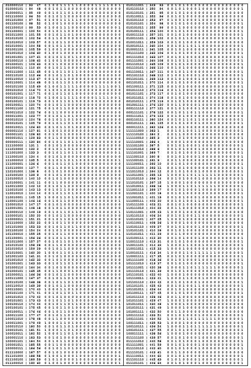
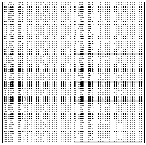
Obviously, the catalog will include 2 ^{3 × 3} = 2 ⁹relations, and each of them will be equipped with a set of inherent properties. Below (Table 3) is a complete list of all 512 relations over the set A, | A | = 3, of three elements. The results of calculating the number of ratios (Table 2), represented by combinations of the numbers of cells of the Cartesian square 3 × 3, of various subclasses for different values ​​of the cardinality of the carrier set (n = 3) are also given. For each relationship, its basic properties and type are indicated (Table 3). The abbreviations used in the catalog are disclosed in Table 2

Table 2. Quantitative characteristics of the catalog for different n





It is convenient to explain the essence of operations with relations and their technique using examples that are especially simple and understandable for binary relations. Operations can involve two and / or more relationships. Operations performed on individual relations are unary operations. For example, operations of reversing (obtaining inverse) a relation, taking a complement, narrowing (limiting) a relation. An example will illustrate how to use the catalog.



Example 2 . Consider the line Npr = 14 of the catalog table. It has the form



The first 9 characters of the line (to the right of the equality) is a binary vector corresponding to a combination of 9 to 2, namely, the number of the first cell (counting from left to right) is the number of the 5th cell of the matrix of the binary relation, i.e. elements a1a1 = a2a2 = 1. This combination has a serial number Ncc = 4 and a through number Npr = 14 in the list of all relations. The rest of this line contains either zeros or ones. Zeros indicate the absence of a property corresponding to the name of the zero column, and ones indicate the presence of such a property in the considered relation.

Properties and quantitative characteristics of relations

Let us consider the most important properties of relations, which will allow us to further highlight the types (classes) of relations used in relational databases in the theory of choice and decision making and other applications. In what follows, we will denote the relation by the symbol [R, Ω]. R is the name of the relation, Ω is the carrier set of the relation.



1. Reflexivity. The relation [R, Ω] is called reflexive if each element of the set is in the relation R with itself (Fig. 2.3). The graph of a reflexive BO has loops (arcs) at all vertices, and the relation matrix contains (E) the unit main diagonal.





Figure 2.3. Reflexive attitude



2. Anti- reflectiveness . The relation [R, Ω] is called antireflexive if no element of the set is in the relation R with itself (Fig. 2.4). Anti-reflective relationships are called strict.





Figure 2.4. Anti-



reflective attitude 3. Partial reflexivity. The relation [R, Ω] is called partially

reflexive if one or more elements from the set are not in the relation R with itself (Fig. 2.5).





4. Symmetry. A relation [R, Ω] is called symmetric if, together with an ordered pair (x, y), the relation also contains an ordered pair (y, x) (Fig. 2.6).





5. Antisymmetry. A relation [R, Ω] is called antisymmetric if, if, for any ordered pair (x, y) є R, an ordered pair

(y, x) єR, only in the case x = y. For such ratios R∩R ^-1 ⊆ E (Fig. 2.7).





6. Asymmetry. A relation [R, Ω] is called asymmetric if it is antireflexive and for any ordered pair (x, y) є R an ordered pair (y, x) ∉ R, for relations R ∩ R ^-1 = Ø (Fig. 2.8).





7. Transitivity. The relation [R, Ω] is called transitive if, for any ordered pairs (x, y), (y, z) є R, in relation R there is an ordered pair (x, z) є R or if R × R⊆R (Fig. . 2.9).





8. Cyclicity. A relation [R, Ω] is called cyclic if for its elements {x1, x2, z3, ..., xn} there is a subset of elements {xi, xi + 1, ... xr, ..., xj, xi}, for which we can write out the sequence xiRxi + 1R ... RxjRxi. Such a sequence is called a cycle or loop (Figure 2.10).





9. Acyclicity. Relationships in which there are no contours are called acyclic. For acyclic relations, the relation R ^k ∩R = Ø for any k> 1 holds (Fig. 2.11).







10. Completeness (connectivity). The relation [R, Ω] is called complete (connected) if for any two elements (y, z) є Ω one of them is in relation to the other (Fig. 2.12). Linearity. Linear relationships are minimally complete relationships.





Figure 2.12. Linear relation



So, we have established that relations, as mathematical objects, have certain properties, the definition of which is given earlier. In the next paragraph, we will consider the essence and manifestation of some properties:

1. Reflexivity x є A (xRx).
2. Antireflexivity x є A ¬ (xRx).
3. Symmetry x, y є A (xRy → yRx).
4. Antisymmetry (xRy & yRx → x = y).
5. Transitivity; x, y, z є A (xRy & yRz → xRz).
6. Cyclicity; x, y є A; ...
7. Completeness x, y є (xRy, yRx);
8. Connectivity (x ≠ y → xRy, yRx).
9. Linearity x, y є (xRy, yRx).

The analysis of the space of relations is a complex task of the theory and, it should be noted, is far from complete. The main results should include the selection of subsets of relations that form complete spaces of relations with all the ensuing consequences.



Quantitative relations of such discrete spaces are of great both

theoretical and practical interest. Some aspects of quantitative characteristics associated with the properties of relations of different types are considered below.

Operations on relations

Like most number systems with relations, the following operations are performed:

• unary;
• binary;
• n-ary.

Below are tables of Boolean ⊕ addition and multiplication & of two variables x1 and x2, mod 2 addition and binary summation:





Above, the concept of a binary relation was introduced, as a subset of ordered pairs of the Cartesian product of sets, and the properties of relations were also considered. In addition, binary relations and matrix representation of relations were mentioned. Let us now consider the concept of a relation in more detail, in addition, consider the basic operations of binary relations, the most important of their set for relations.



For them, the following conditions must be met:

• The arity of the operands in the operation must match;
• the result of the operation must be a relation of the same arity.

For binary and n-ary relations, the following must be satisfied: the arrival area of ​​the first operand must match the origin area of ​​the second operand.



Unary operations on relations



Inversion of relations . The inverse of the relation R is the ratio R ^-1 , defined by the condition xR ^-1 y <=> yRx. More correctly, this operation should be called pseudo-inversion, since p · p ^-1 ≠ E = Δ.



Let the relation be written in the form of listing the ordered pairs included in it. If in each pair the components are interchanged, then the new pairs form the ratio P ^-1 , which is called the inverse to P.



The inverse relation to the relation P is the relation formed by the pairs (ai aj) for which (aj ai) є P ^-1 . For relations in matrix form, inverse relations are obtained by transposition of the matrix P.



9. The dual relation (P ^d ) to the relation P is the relation formed by all those pairs that belong to the universal relation and do not belong to the inverse relation (addition to the inverse):



P ^d = {(ai aj) | ((ai aj) єA × A) & (ai aj) ∉ P ^-1 )} = (A × A) \ P ^-1 .



The dual and inverse relations in the aggregate contain all pairs of the Cartesian product A × A and do not have common pairs, they, like the relations P and P form a partition A × A





Note that for any relation P is not satisfied P P = ^d .



Narrowing (PA1). The relation [R1, A1] is called the restriction of the relation [R, A] to the set Ω1 if Ω1⊆ Ω and R1 = R∩Ω1 × Ω1. The ratio PA1 on the set A1 ⊆ A is the ratio PA1 on the set A1, formed by all those pairs that belong to the relation P and are simultaneously part of the Cartesian product A1 × A1. In other words, PA1 is the intersection of the relations P and A1 × A1. Let A1 = {a1, a3, a4}, then for the relations P and Q in matrix form, the narrowing relations will have the form:





Binary Operations



Operations requiring at least two relations are n-ary (n-ary). Only relations of the same arity can participate in such operations. Examples of such operations: intersection, union, difference, symmetric difference of relations, and some others. If the operation uses more than two relations, then it is performed sequentially for the first two, and then for the final relation and the third, etc.



In other words, these operations are defined for two relations. In operations on relations, it is assumed that the domains of specifying relations (operands and the result) coincide, the arities of the relations coincide, and the result of the operation is again a relation of the same arity. As examples, we will consider operations on binary relations P and Q defined on a discrete set

= {a1, a2, a3, a4} by Boolean matrices (as a rule, zeros do not fit into the matrix):





1. Intersection (P ∩ Q) is a relation formed by all those pairs of elements from A that are included in both relations, ie common to P and Q,

P ∩ Q = {(ai aj) | ((ai aj) є P) & ((ai aj) є Q)}.



The ratio matrix P ∩ Q is obtained as the Boolean intersection of the matrices P and Q:





In the absence of such common pairs, the intersection of relations is said to be empty, i.e. it is a null-relation. The intersection of the relations R1 and R2 (R1∩R2) is the relation determined by the intersection of the corresponding subsets from A × A.



2. Union (PUQ). The union of the relations R1 and R2 (R1UR2) is the relationship defined by the union of the corresponding subsets from A × A. The ratio formed by all the pairs that make up either the ratio P or the ratio Q, i.e. by pairs belonging to at least one of the relations (the connective ∨ - or the unifying one)

PUQ = {(ai aj) | ((ai aj) є P) ∨ ((ai aj) є Q)}.



If in the set A × A there are no other pairs that are not included in the relation PUQ, and their intersection is zero, then the relations P and Q are said to form a complete relation A × A when combined, and their system is a partition of this complete relation. The union of the relationship matrices is formed as a Boolean sum of the relationship matrices:





3. The difference (P \ Q) is the ratio formed by those pairs from P that are not included in the relation Q

P \ Q = {(ai aj) | ((ai aj) є P) & ((ai aj) ∉Q)}.



The difference for relations in matrix representation is





4. Multiplication of relationships. Ordered pairs forming a relationship may or may not contain the same elements. Among the pairs that have identical elements in their composition, let us single out such ordered pairs, which we call adjacent (adjoining) and which have the 1st element in the second pair, and the 2nd element in the first pair is the same. Let's define the product of adjacent pairs as an ordered pair:

(ai ak) ∙ (ak aj) => (ai aj).



In terms of graph theory, the above means that adjacent pairs form a route from point (ai) to point (aj) in transit through point (ak), consisting of 2 adjacent arcs. The product of these arcs is the third arc from point (ai) to point (aj), which implements the transition between the extreme points of the route in the same direction, bypassing the intermediate point (ak). The arc (ai aj) is said to close these points directly.



5. Symmetric difference (P∆Q) - the ratio formed by those pairs that are included in the union PUQ, but are not included in the intersection P∩Q. Another form of definition explains the name of the operation: P∆Q is formed by those ordered pairs that are the union of the differences P \ Q and Q \ P. Thus, the expression for the symmetric difference is written in two different ways:

P∆ Q = (PU Q) \ (P ∩ Q) = (P \ Q) U (Q \ P).



The symmetric difference matrix is:





From the last record it follows that the operation of symmetric difference allows permutation of the operands, that is, it is commutative.



5. Composition or product (P ∙ Q) - the relation formed by all pairs for which:

P ∙ Q = {(ai aj) | ((ai ak) є P) & ((ak aj) є Q)}.



In other words, each ordered pair in the resulting relation is the result of multiplication of adjacent pairs, of which the 1st pair belongs to the first factor-relation, the 2nd - to the second factor-relation. The composition operation is not commutative.



Composition (◦Q) on a set M is a relation R defined on the same set M that contains a pair (x, y) when there exists Z є M such that (x, z) є P and (z, y) є Q.



In the matrix representation of relations, the composition matrix of relations is equal to the Boolean product of the matrices of the original relations:





A special case of the composition of relationships is the square of the relationship.



It can be shown using induction that the nth degree of a relation is defined recursively by the formula: P ⁿ = P ^n-1 ◦, this means that the pair (x, y) є P ⁿ in the case when in the matrix there is a chain elements: such that (xi, xi + 1) є P, 1 <i <n – 1.



The composition operation has the property of associativity (like a product of matrices).



The composition of relations on the set M is the result of a pairwise composition of relations for any arrangement of parentheses. The area for setting the composition result does not change.



Composition for Boolean matrices of relations is formed as a result of the Boolean product of matrices of these relations.



Table 3. Catalog of binary relations (n ​​= 3). Clickable